MolArch+ - General Commands MolArch+ - General Commands |
- help [command] [keywords]
- manual [command] [keywords]
|
-
Display information about a specific command and/or its options
contained in the 'molarch+.hlp' file.
|
|
-
Display short syntax information about a specific command and/or its
options that is contained in the 'molarch+.syn' file.
|
|
-
Display commands and options matching up to three keywords specified.
|
|
-
Show history of commands. If '[keywords]' are specified, only the matching
commands are listed. If a history number '<n>' (either positive or negative
number) is specified, the corresponding command is executed.
|
|
-
These synonymous commands execute the last command matching a given list of
(maximum three) keywords. If a history number '<n>' is specified, these
commands behave just like the 'history' command itself.
|
|
-
For use in external, executable scripts (SPR-files) only: stops
execution, 'stop' is not an interactive command.
|
|
-
Quit program (somehow self-explanatory, or?), 'quit' and 'bye' also
clean up temporary files used by molarch+ (TMP_*.*), whereas 'exit'
leaves these files untouched.
|
|
|
|
-
The key-sequences 'escape 1' to 'escape 9' can be set-up as short-cuts
for any command including any number of options. Simply press the
'escape'-key followed by '1' - '9' to execute the corresponding command.
-
If an invalid key is pressed after 'escape', a list of short-cuts
available is displayed. The key sequence 'escape 0' can be used to
repeat the previous command, i.e. when going through a sequential
PDB-file using the 'next' command, simply press 'escape 0' to step
to the next structure.
|
- wait {key, mouse, event, <count>}
|
-
Wait for an event (pressed key and/or mouse click) or for a given time
<count> (no units, simply test it!).
|
MolArch+ - Loading Files (Import) |
- pdbload <filename> [<molnum1>] [<molnum2>]
|
|
|
-
Load only the first molecular structure (file format is Protein Data Base)
from a sequential PDB-file (multiple HEADER records). If the PDB-file actually contains more than
one molecular structure, all except the first are ignored.
|
- outload <filename> [<molnum1>] [<molnum2>]
- macload <filename> [<molnum1>] [<molnum2>]
- macromodel <filename> [<molnum1>] [<molnum2>]
|
-
Load MacroModel OUT- and MAC-files;
for comments on '<molnum1>' and '<molnum2>'see 'help pdbload'.
|
- dg <filename> [<molnum1>] [<molnum2>]
- dgload <filename> [<molnum1>] [<molnum2>]
|
-
Load DG-files from distance geometry calculations;
for comments on '<molnum1>' and '<molnum2>'see 'help pdbload'.
|
|
-
Both (identical) commands 'hinload' or 'hyperchem' try to read and load
molecular structures from Hyperchem HIN-files.
|
- p88load <filename> [<molnum1>] [<molnum2>]
- ampload <filename> [<molnum1>] [<molnum2>]
|
-
Load atom-mapped properties and molecules from an input-file. These
'*.amp' files include a molecular geometry, the bond list, atomic charges
(total, sigma, and pi-charge), and split terms of energy (bond, angle,
torsion, bend, coulomb, and vdw). To map the individual properties
onto a molecular model use the 'property' command and its numerous options.
-
The 'ampload' and 'p88load' are synonyms, as the PIMM output files
'*.out' or '*.log' may be read and analyzed with both of these 'commands'.
Older versions of PIMM (PIMM88) did include the atomic split terms of
energy in their output files, newer versions may not do so.
-
To save files in this format, use 'save amp <filename>', to calculate
the split terms of strain energy see 'help strain'.
|
- rdfload <filename> [<molnum1>] [<molnum2>]
|
-
Load Isis-Draw RDF-files (chemical formulas, experimental only).
|
|
-
Load a molecular structure with free file format. The file can contain
more than one molecule, lines with less than 12 characters are
considered as separators (very much like the HEADER records in a PDB
file), they represent the title lines. If only one title line starting
with 'E' is found at the beginning of the file, the columns 2-11 of this
line are converted into an energy value of the molecule, that will also
appear when saving the molecules into a PDB file.
Atom labels start left justified in column 1 (upper and lowercase
letters allowed), the coordinates follow in free format separated by at
least one blank each (e.g. 'Zn -1.3478 3.4873 5.6659').
|
|
-
Load bondlist, angle and torsion angle definitions from CHARMM molecular
topology file (psf-format).
|
|
-
Load CHARMM molecular structure file.
|
|
-
Load atomic charges (atom sequence must correspond to current PDB-file).
|
|
-
Load a PIMM91 input-file (*.ein: Cartesian or internal coordinates)
or an output-file (*.opt: Cartesian coordinates only!).
|
|
-
Load a molecular surface (file format is MOLCAD) and delete previously
loaded surface data (see also the command 'addsurface').
|
|
-
Load a 3D-contour file generated by the program 'molcont+' as a
surface. The contour files can also be uploaded with the 'sldload'
and 'addsurface' commands.
|
|
-
Load a second, third, ... molecular surface (file format is MOLCAD).
Multiple files may be loaded simultaneously by giving multiple filenames
or by using wildcards ('*' and '?'), e.g. 'addsurface *.sld';
previously loaded surface are kept.
|
|
-
Load a fragment definition file.
|
|
-
Load a definition file for molecular topologies (see also command
'save fragment').
|
|
-
Load a molecular topology file - This is a file containing atomic numbers
describing molecular fragments. After a successful 'search' of molecular
fragments, use 'save topology <filename>' to generate a template file which
may be edited. Then use 'topology <filename>' to reload the file.
|
|
-
Load a RC-file containing user defined settings of display parameters.
At start-up time, MolArch+ looks for a file '$MOLARCH/molarch+.rc' and reads
the settings from it. If this file is copied into the working directory or
your $HOME directory, it may be used to override the built-in settings of
MolArch+ or those defined in '$MOLARCH/molarch+.rc'.
-
For details see the system parameter file '$MOLARCH/molarch+.rc' and the
comments at 'help save rc'.
|
|
-
Execute a batch file - All settings and program options
could be stored in a batch file that can be executed with
this commend. By editing this ASCII (readable) file
animations and automated demonstrations can be generated.
(see also command 'save spr <filename>'). 'sprload' explicitly
'sets quiet on', that is no molecular surfaces are displayed
while loading the SPR-file. This can be overridden by 'setting
quiet off' as the first command within the SPR-file.
|
|
|
|
|
|
-
Load thermal anisotropic ellipsoids (*.ell must match PDB-file).
(see also commands 'set ellipsoids', 'set cut-ellipsoids',
and 'set hatching').
|
|
-
Toggle the display of thermal anisotropic ellipsoids (if available).
|
- DATLOAD or
- datload <filename> [set <configuration>] [single] [shift-molecules, shift] [center-molecules, nocenter] [all-positions, asymmetric-units, original-positions] <xcells> <ycells> <zcells>
|
|
- cpimmload <filename> [single] [set <configuration>] [shift-molecules, shift] [center-molecules, nocenter] [all-positions, asymmetric-units, original-positions] <xcells> <ycells> <zcells>
|
|
- cifload <filename> [single] [shift-molecules, shift] [center-molecules, nocenter] [all-positions, asymmetric-units, original-positions] [probability <value>] [ellipsoids] [type <n>] <xcells> <ycells> <zcells>
|
-
Load SHELX-crystallographic files (fractional atomic coordinates, unit
cell data, and thermal motion probability ellipsoids).
-
For a description of most of the options see 'help datload'.
The 'probability <value>' option allows to read the isotropic and anisotropic
thermal ellipsoids from the SHELX-file (if included). The ellipsoids are
scaled to visualize a specific <value> of the probability contours, whereas
the probability value may be give in the range of 0.01-0.99 (or alternatively
1-99%). The standard description for anisotropic thermal ellipsoids used by
SHELX corresponds to the ORTEP-III type no. 8 (U11, U22, U33, U12, U13,
and U23), this type can be changed with the 'type <n>' option. For more
details, please refer to the SHELX and ORTEP manuals (see the reference
of the 'molarch+.hlp' file). The 'ellipsoids' option is simply a synonym
for the keywords 'probability 50%'.
-
Please note: each SHELX-file contains one dataset only, therefore the
'[set <configuration>]' option which is valid with CCDF-files cannot be
used here.
|
- logload <filename> [mulliken-charges, natural-charges]
|
-
Load Gaussian LOG-files (output files; Cartesian coordinates and atomic
charges) - see also 'help g94', and 'help fcheck'. Currently, Gaussian94
and Gaussian98 files are supported. Use the keywords 'mulliken-charges'
or 'natural-charges' to specify which set of atomic charges should be
read from the LOG-file (default behavior is to keep the last set of charges
in the LOG-file irrespective of their type).
|
- spartan-load <filename> [esp-charges, mulliken-charges, npa-charges]
|
-
Load a Spartan file - if one of the key words 'esp-charges',
'mulliken-charges', or 'npa-charges' is given, the corresponding charges
are extracted from the file, too.
|
- dhxload <dhx-file> [<configuration>]
- dcdload <dcd-file> [<configuration>]
|
-
Load a CHARMM MD molecular structure (ASCII encoded binary format, or
BINARY files).
Since these files do not contain information about atom types, a
corresponding molecular structure must have been loaded previously
from an independent source file (e.g. a PDB-file).
If <configuration> is stated, the corresponding geometry is read from
the file, otherwise the first molecular arrangement is loaded.
|
|
-
Load a CHARMM MD restart file: first load the molecular topology
and atom types from an existing PDB-file (same basename, extension
'.pdb') - then load the coordinates from the restart file according to
<mode>:
<mode> < 0 : load coordinates from XOLD, YOLD, ZOLD dataset.
<mode> = 0 or 1 : load coordinates from X, Y, Z dataset.
<mode> > 1 : load both coordinate sets (doubling the number of atoms).
<mode> = -1, +1 : load only solute coordinates (delete all water molecules,
and load coordinates from XOLD, YOLD, ZOLD or X, Y, Z) and show actual
velocities as thermal ellipsoids.
|
- DHXLOAD <pdb-file> <dhx-file> [<configuration>]
- DHXLOAD <pdb-file> <dhx-file> sequence <pdb-output-file>
|
-
Load a CHARMM MD molecular structure (ASCII encoded binary format).
Since these files do not contain information about atom types, a
corresponding PDB-file must be loaded simultaneously (two filename are
required), the atomic labels are read from the PDB-file, whilst the
coordinates are extracted from the DHX-file.
If <configuration> is not stated, only the first molecule is loaded.
The 'sequence' option sequentially loads all configurations contained
in the CHARMM file, and saves them to a <pdb-output-file>. For further
information on the DHX-file format, please refer to the CHARMM manuals.
|
|
-
Similar to command 'datload', but LEMMI's own data format (long time
before 'datload' worked properly ...). For further information see
'help unit-cell'.
|
- cubload <filename>
- cubload <filename> [multiple options]
- cube calculate [multiple options] [additional options]
|
-
[multiple options] can be:
[grid <n>]
[cmap {esp, mep, mlp, gry, red, green, yellow, blue, magenta, pink, cyan, white, <colornum>}]
[contours <n>] [align-grid]
[crop-grid <value>] [xcrop-grid <value>] [ycrop-grid <value>] [zcrop-grid <value>]
[skip-points <n>] [default <value>] [minimum <value>] [maximum <value>]
[exclude-surface] [area-min <value>]
[combine-contours <n>] [transparency <value> <value> <value>]
[color-scale <value>] [red <value> [value]] [green <value> [value]] [blue <value> [value]]
-
[additional options] are:
[mode {esp, mep}] [molecule <molnum>]
[points <n>] [xpoints <n>] [ypoints <n>] [zpoints <n>]
[step <value>] [xstep <value>] [ystep <value>] [zstep <value>]
[size <value>] [xsize <value>] [ysize <value>] [zsize <value>]
[offset <value>] [xoffset <value>] [yoffset <value>] [zoffset <value>]
-
Loading molecular structures from a Gaussian cube-file is simply done by
using the command 'cubload <filename>' without any additional options.
If a read error occurs, please note that these files must contain exactly
two title lines, the rest of the input format is described in the
corresponding Gaussian manuals.
-
However, Gaussian cube-files generally contain 3D grids onto which Gaussian
has mapped atomic or molecular properties. MolArch+ may be used to also
import this data and convert it into transparent 3D densities representations
when used with high-quality external rendering programs such as POVRAY. The
cube data may also be mapped onto molecular surfaces or any other surface
object (see 'help qadd' and 'help quality').
-
Except for the format of the file imported and the 'grid <n>' option
(see below), the 'cubload' command accepts the same options and keywords
as the 'field-load' command. For a detailed description of these very
complex options see 'help field-load'; these help pages contain informations
which are of particular importance if the cube data is to be used with
POVRAY renderings of 3D transparent contours, or if MolArch+ should color
grid data according the range of property values on the grid. Read the
'help field' pages carefully.
-
If the grid data of the cube file should be imported by MolArch+, the 'grid'
option below MUST be given. Otherwise this part of the file is ignored and
only the molecular structure information contained in the header section of
the cube file is read.
-
If the cube grid has to re-exported by MolArch+, see 'help save cube' or
'help save field' (this command uses a different file format).
-
[grid <n>]
If the 'grid <n>' option is given, the data of the <n>-th grid contained
in the cube-file is read (e.g. density, orbital, or potential data). This
data maybe used to add surface qualities using the 'qadd' command
(e.g. add density qualities or electrostatic potentials on Connolly-type
molecular surfaces); or to produce 3D renderings of the data by POVRAY.
For cube grid files containing only one field of data the 'grid 1' option
must be used, for cube files which contain multiple Gaussian grids the
corresponding grid number '<n>' must be specified (e.g. 'grid 2').
Invalid grid numbers result in error messages. In general, MolArch+ can
handle only one grid of properties at the same time.
By reading a specific grid data field and re-exporting a cube file
(see 'help save cube') MolArch+ may be used to split Gaussian multiple-grid
files into single-grid cube files.
-
[calculate]
If the 'calculate' option is used as the first argument to the 'cube'
(or 'cubload') command (i.e. if this keyword is used instead of a '<filename>'
argument), MolArch+ is instructed to generate a new grid of properties
around the currently active molecule(s). This command is synonymous to the
the command 'field calculate ...', and all additional options applicable to
this command are listed in the corresponding help section available from
'help field'.
|
- field-load <filename> [multiple options]
- field calculate [multiple options] [additional options]
|
-
[multiple options] can be:
[cmap {esp, mep, mlp, gry, red, green, yellow, blue, magenta, pink, cyan, white, <colornum>}]
[contours <n>] [align-grid]
[crop-grid <value>] [xcrop-grid <value>] [ycrop-grid <value>] [zcrop-grid <value>]
[skip-points <n>] [default <value>] [minimum <value>] [maximum <value>]
[exclude-surface] [area-min <value>]
[combine-contours <n>] [transparency <value> <value> <value>]
[color-scale <value>] [red <value> [value]] [green <value> [value]] [blue <value> [value]]
-
[additional options] are:
[mode {esp, mep}] [molecule <molnum>]
[points <n>] [xpoints <n>] [ypoints <n>] [zpoints <n>]
[step <value>] [xstep <value>] [ystep <value>] [zstep <value>]
[size <value>] [xsize <value>] [ysize <value>] [zsize <value>]
[offset <value>] [xoffset <value>] [yoffset <value>] [zoffset <value>]
-
This command allows to import 3D grid data of spatial properties around
molecules (i.e. 3D grids which have been superimposed to a molecule, for
which at each grid point a quality or property was calculated). This grid
data may be used to generate transparent color-coded 3D maps of e.g.
electrostatic potentials, electron densities, etc. around molecules.
Although MolArch+ uses only simplified methods to visualize the grid data
with limited options only, these 3D densities are saved with high-quality
in VRML and POVRAY scenes; which may be used to generate high-resolution
images and/or animations (see 'help save wrl' and 'help save pov'). The
grid data may also be mapped onto molecular surfaces or any other surface
object (see 'help qadd' and 'help quality' for the 'cube' keywords).
-
This command reads ASCII files with a simple MolArch+ specific format
(CON-files). Files of this type may be generated by importing Gaussian
cube files (see 'help cubload') or by the command 'field calculate ...'
(see below), and saving the data obtained with 'save field <filename>'.
In the 'examples' directory you will find some typical grid files '*.CON',
the file format is simple and may easily be generated from other
sources, too.
-
Gaussian cube files contain data similar to the CON-files used by this
command, and all options of the 'field-load' command apply also to the
'cubload' command which is used to read the Gaussian files.
-
Use the command 'set unit-cell {on, off}' after the grid was imported, to
display a unit-cell like bounding box indicating the dimensions of the
3D grid. The display of the grid data itself can be toggled using the
command 'set {grid, field} {on, off}'.
-
MolArch+ offers the possibility to calculate molecular properties
such as the molecular electrostatic potential on 3D grids.
See below for the 'calculate' option.
-
If the grid data is to be included into high-resolution POVRAY graphics
as transparent contours, several display options must be set at the
time the field data (or Gaussian cube data) is read, currently there is
no possibility to change these settings latter except by re-loading the
grid data with other options as appropriate. The options below are NOT
considered if the grid data should be mapped onto other (molecular)
surface objects.
-
The following options SHOULD be set with this command if the grid data
is to be used with POVRAY:
-
[cmap {esp, mep, mlp, gry, red, green, yellow, blue, magenta, pink, cyan, white, <colornum>}]
The 'cmap' option defines the color-map which is used to visualize
the 3D properties or densities. For details on color scales used by MolArch+
see 'help map' and 'help cmap'. It is important to note, that the
transparency and color parameters used with the grid data are read from
the corresponding color definitions files. Informations on these files
is obtained by the command 'molarch- -Sneo --quit'.
These color scales may need editing for each 3D grid of data and
appropriate transparency values must be defined (the POVRAY renderings
are highly sensitive to the transparency values!). Copy a color
file from the '$MOLARCH' directory to a new local color definition file,
edit it, and load the color definitions (see 'help cmap') prior to the
'field-load' or 'cubload' command.
The keywords 'red', 'green', 'yellow', 'blue', 'magenta', 'pink', 'cyan',
and 'white' indicate that all grid points are plotted with the same color
as specified (this may not be really particularly useful).
-
[contours <n>]
The number of color contours to draw should be specified (i.e. the number
of of color shades used to map the grid data; the default value '<n>' is
the number of color shades in the color scale defined by the 'camp' option).
A high value of '<n>' corresponds to a high resolution of the color scale on
the cost of larger rendering files. Try values in the range of 8-16.
-
It is HIGHLY recommended to use the following options if the grid data
is to be included into POVRAY scenes:
-
[align-grid]
The 'align-grid' uses an advanced and faster algorithm to save 3D grid
data with POVRAY files for rendering. In this case, the grid data is
aligned with the current window coordinate system at the moment the POVRAY
file is saved. This option MUST also set the 'crop-grid' option (see below).
It is also highly recommended to use the command 'set texture on' to
enable a fast graphics mode (use this command before or after the 'field'
command, for further informations see 'help set texture').
-
[crop-grid <value>] [xcrop-grid <value>] [ycrop-grid <value>] [zcrop-grid <value>]
This option should be used to exclude outer grid regions (which are far
away from the molecule of interest in the center of the grid). At
the time high-quality rendering POVRAY files are produced, parts of the
3D grid which are more than '<value>' Angstroms apart from the central
molecule are discarded; the 'xcrop-grid', 'ycrop-grid', and 'zcrop-grid'
keywords allow to adjust the displayed grid size independently in the
x-, y-, and z-direction.
At least one of these 'crop' options MUST be used with the above mentioned
advanced and faster algorithm to save 3D grid POVRAY contours (see option
'align-grid').
-
The following options are likely to be useful if the grid data
is to be included into POVRAY scenes:
-
[skip-points <n>] [default <value>]
Of the 3D grid contained in the CON-file or the Gaussian cube file,
a number of <n> points is skipped on the front, back, left, right,
top and bottom side. Large values <n> will load only small center
sections of the 3D grid. Apply large values first for test cases, then
slowly decrease <n> until the box has the desired size. Too large grids
may result in too big contour files with POVRAY.
If <n> is a negative integer, the 3D grid is not cropped, but expanded
by the absolute value of <n> number of points. The 'default' value '<value>'
is assigned to all additionally created grid points.
For 'cropped' grids it is not recommended to load only parts of the
original contour file ('skip-points <n>' with <n> greater than 0), but
it may be necessary to expand the original data set using the options
'skip-points <n> default <value>' with <n> less than zero (cf. above).
-
[minimum <value>] [maximum <value>]
By default, the color scale used to display the 3D grid data (see above)
is adapted to the range of property values found on the grid. With these
'minimum <value>' and 'maximum <value>' options this range of values
may be defined by the user. Grid points with properties less than
'minimum' will be assigned to the lowest color shade available, those
with values larger than 'maximum' will be mapped onto the highest color
shade (see 'cmap' option above and command 'map').
These options may stretch or compress the color scale in relation to
the range of values on the grid. Any user specified boundary overrides
the range of values found on the actual grid.
-
[exclude-surface]
If this option is enabled and if a molecule including any surface
(molecular surface, etc.) is active at the time the grid data is read,
all grid points contained in the inner volume of this surface are
discarded. The inner volume of molecular surface is defined by the
surface normal vectors and the surface triangles (see 'help normals'
and 'help triangles'). With large grids and large surfaces this
may take some computational time.
This option is particularly useful if electrostatic potentials have to
be mapped around molecules, as these potentials have very large negative
or positive values close to the positions of the nuclei of the molecule(s).
With the aid of molecular surfaces (e.g. Connolly-type or solvent-accessible
surfaces) these regions may be ignored for rendering and for adapting
the color scales (grid property values inside of surface are not used
when calculating the minimum and maximum property values on the grid).
-
[area-min <value>]
This expert-mode parameter may only be used to limit the resolution of the
3D contours. Usually contour triangles are not saved if their area is less
than <value> (default is 1% of the grid resolution), and generally there
is little need to change this parameter.
-
The following options are DEPRECIATED or RARELY useful as they define the
color scales via mathematical functions (old method):
-
The options below may be useful only if the grid data contains something
like relative water densities around a central molecule in solution:
The relative water densities are mapped onto a color scale ranging from
blue (standard bulk phase water density) over yellow to red (enhanced
water densities). The number of color shades, their relative colors and
the resolution with which the grid contours are calculated can be varied
with the following parameters:
-
[combine-contours <n>]
The first <n> contours (which may only describe the bulk phase water) may
be combined into one contour without the loss of much information, but
resulting in much smaller files. The bulk of grid points resides in the water
outer water phase, and it is recommended to use an value of <n>=1
(default=0), and the first two contours are by far the biggest (in terms
of color information) to save.
-
[transparency <value> <value> <value>]
The two values describe the transparency (<value>=0.0: completely opaque,
and <value>=1.0 completely transparent) of the water density contours, the
first value refers to the bulk phase (blue) water contours, the latter
value corresponds to the regions of high water density (red). Recommended
is a value of approx. 0.950-0.975 for the bulk phase transparency (note
that the optimum of this value depends on your grid size, it is very
sensitive to small changes and should be varied very carefully in small
steps). A transparency value of 0.20-0.50 is recommended for the red, high
density contours (this value is less sensitive and may be varied over a
larger range). The last (optional) value may be used to change the dependency
of the transparency on the grid values (linear: <value>=1.0, squared: 2.0,
and so on).
-
[color-scale <value>] [red <value> [value]] [green <value> [value]] [blue <value> [value]]
The standard color-scale used to draw the 3D water density contours (in
the range of x=0.0 (bulk phase) to 1.0 (highest density)) a combination of
3 functions:
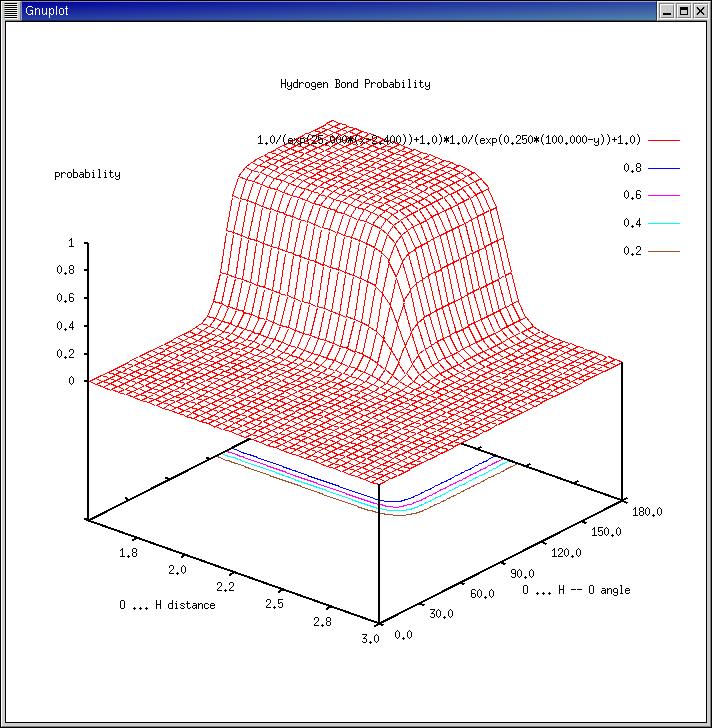
red: 1.0/(exp( 25.0*(0.30-x))+1.0) Increasing Fermi-Dirac type function.
green: exp(-75.0*(0.40-x)**2) Gaussian function.
blue: 1.0/(exp( 25.0*(x-0.30))+1.0) Decreasing Fermi-Dirac type function.
(yellow corresponds to the product of red*green). Please use a plot
program like 'gnuplot' to plot the scale:

|
  set yrange [0.00:1.25]; set xtics 0.0,0.1,1.00
  set xrange [0.00:1.00]; set ytics 0.0,0.1,1.00
  plot   1.0/(exp( 25.0*(0.30-x))+1.0)
  replot      exp(-75.0*(0.40-x)**2)
  replot 1.0/(exp( 25.0*(x-0.30))+1.0)
  replot 1.0/(exp( 25.0*(0.30-x))+1.0)*exp(-75.0*(0.40-x)**2)
|
The above 'color', 'red', 'green', and 'blue' keywords may be used to
modify the following default parameters:

|
  set yrange [0.00:1.25]; set xtics 0.0,0.1,1.00
  set xrange [0.00:1.00]; set ytics 0.0,0.1,1.00
  red1   = 0.30;   red2   =  25.0
  green1 = 0.40;   green2 = -75.0
  blue1  = 0.30;   blue2  =  25.0
  plot   1.0/(exp(  red2*(red1  -x))+1.0)
  replot exp(green2*(green1-x)**2)
  replot 1.0/(exp( blue2*(x-blue1 ))+1.0)
  replot 1.0/(exp(  red2*(red1  -x))+1.0)*exp(green2*(green1-x)**2)
|
In general, the use of the 'color' command is to be preferred, since it
only moves the transition zone blue-to-yellow-to-red to larger or small
values (default 0.30, recommended 0.20-0.40). Higher values increase the
blue contours, lower values increase the yellow and red contour parts.
-
The following options are used to generate 3D grids around molecules or
molecular assemblies:
-
[calculate]
If the 'calculate' option is used as the first argument to the 'field'
(or 'field-load') command (i.e. of this keyword is used instead of a <filename>
argument), MolArch+ is instructed to generate a new grid of properties
around the currently active molecule(s). This command is synonymous to the
the command 'cube calculate ...', and all additional options listed below
apply to both commands (see also 'help cubload').
-
[mode {esp, mep}] [molecule <molnum>]
This option allows to specify what has to be calculated on a 3D grid
superimposed to the currently active molecule(s). Currently only the
calculation of molecular electrostatic potentials ('mep') is supported
(identical to 'esp'); future releases may include more properties.
The 'mep' (or 'esp') mode require a molecule or set of molecules
to be loaded with appropriate atomic charges, MolArch+ will compute the
electrostatic potential (Coulombs law) on each grid point around the
molecule.
If the potential has to be calculated only for one molecule (and its charges)
out of a set of many molecules, use the option 'molecule <molnum>' to
specify a single molecule. If not specified otherwise, the over-all
(total) electrostatic potential is generated using all molecules and their
atomic charges available on display.
The options below are used to indicate the dimensions and resolution
of the 3D grid that is superimposed to the molecule(s). Of these options
several pairs (e.g. number of grid points and offset, or grid size and step
size) may be used to fully specify the grid parameters; any invalid
specification results in an error message:
-
[points <n>] [xpoints <n>] [ypoints <n>] [zpoints <n>]
Number of grid points in either all directions or independently in x-, y-,
and z-direction (relative to the molecules in their original orientation on
file). The 'points' options simultaneously set the 'xpoints', 'ypoints'
and 'zpoints' options to equal values.
-
[step <value>] [xstep <value>] [ystep <value>] [zstep <value>]
Spacing between grid points (step size) in each direction (in Angstroms).
-
[size <value>] [xsize <value>] [ysize <value>] [zsize <value>]
Absolute size of the 3D grid in any direction (in Angstroms).
-
[offset <value>] [xoffset <value>] [yoffset <value>] [zoffset <value>]
Distance between outer grid border and all molecule(s) in any direction
(in Angstroms).
|
|
-
The 'next' command gets the next molecular structure from a sequential
PDB-file ('NEXT' includes recalculation of the bondlist), and so on.
The commands 'next' and 'NEXT' also work for CHARMM DCD- and DHX-files,
MACROMODEL OUT- and MAC-files, CCDF x-ray data files (FDAT), and distance geometry (DG) files.
|
MolArch+ - Saving Files (Export) |
- save pdb <filename> [<molnum1>] [<molnum2>]
- save PDB <filename> [<molnum1>] [<molnum2>]
|
-
Save a molecular structure as PDB-file in the original orientation
(see 'save new <filename>'). Atoms are stored in molecular order.
If 'PDB' is capitalized, atoms are stored in the original order and
a bond list is included (CONNECT records of the PDB-file).
If <molnum1> is specified, only the atoms of the specified molecule
are stored, if <molnum1> and <molnum2> are given, only the
molecules starting from <molnum1> up to <molnum2> are saved.
|
- save macromodel <filename> [<molnum1>] [<molnum2>]
- save MACROMODEL <filename> [<molnum1>] [<molnum2>]
|
-
Save a structure as a macromodel input file - only appropriate if
the molecular data was already loaded from a macromodel file.
If the capitalized keyword 'MACROMODEL' is used, the molecules are
saved in the current orientation.
|
- save esp <filename> [<molnum1>] [<molnum2>]
|
-
Save all atomic charges into an ESP-file.
|
- save new <filename> [<molnum1>] [<molnum2>]
- save NEW <filename> [<molnum1>] [<molnum2>]
|
-
Save a molecular structure as PDB-file using the current (i.e.
translated, rotated, and scaled) coordinates. The capitalized option
'NEW' has the same effect as in 'save PDB'.
|
|
-
Save a molecular structure and all atom-mapped properties to a external
file. The file includes atomic coordinates and the bond list, the
atom-mapped properties include total-, sigma-, and pi-charges,
split terms of energy (bond, angle, torsion, bend, coulomb, and vdw).
The command 'save AMP <filename>' saves molecules in the the current
orientation.
-
To re-read these files use 'ampload <filename>'. For the use of
atom-mapped properties see 'help property'.
|
- save ein <filename> or: save pimm <filename>
- save EIN <filename> or: save PIMM <filename>
|
-
Save a molecular structure as input-file for the force-field
program PIMM91 (H.J.Lindner, M.Kroeker, PIMM91 - Closed Shell
PI-SCF-LCAO-MO-Molecular Mechanics Program, Technical University
of Darmstadt, 1991). CHECK HEADER PARAMETER and PI-SYSTEM for
calculation.
-
The option 'ein' or 'pimm' saves the atoms in molecular with
Cartesian coordinates.
-
The option 'EIN' or 'PIMM' tries to save internal coordinates.
If a definition table was obtained from the last 'pimmload'
or 'optload'-command it is used for output; otherwise, molarch+
will try to build a new one. If not successful, Cartesian
coordinates are saved. See also the 'sort' command, in
particular the 'sort all' option.
-
ATTENTION: Once a PIMM-file has been loaded and the
structure was edited subsequently, use 'set pimm' to force
a re-definition of atomic-types! Otherwise, the original atomic
types obtained from the PIMM-files are used and PIMM may add
undesired hydrogens or crash.
|
- save g94 <filename> or: save gaussian <filename>
- save G94 <filename> or: save GAUSSIAN <filename>
|
-
Save a molecular structure as input-file for Gaussian (Cartesian
coordinates only). Edit the job and/or charge and spin multiplicity
parameters manually. The capitalized keywords save the molecule in
the current orientation, 'g94' or 'G94' tries to write internal atomic
coordinates ('z-matrix'), whereas 'gaussian' or 'GAUSSIAN' save Cartesian
atomic coordinates only.
|
|
-
Save crystal data in a Cambridge Crystallographic Data Center analog file
format (not exactly), which can reloaded by molarch+ using the 'datload'
command. This command requires that some crystal data was read in from
a CCDF-file or a SHELX-file (see 'help datload' or 'help cifload').
Preferably, only the asymmetric unit should be loaded before applying
the 'save dat-file' command (this unit may be edited before saving!).
This asymmetric unit is saved together with unit cell dimensions, symmetry
operations, bond-list, and atom informations; thermal anisotropic ellipsoids
are discarded.
|
- save cpimm-file <filename>
|
-
Save crystal structures as input files for the force-field program PIMM.
The prerequisites are analog to the 'save dat-file' command (see also the
corresponding help file).
|
- save {fragment, parameter, sub-structure} <filename>
|
-
Save the molecular topology obtained from a 'sub-structure'
definition (see the command 'sub-structure').
|
|
-
Save the results from a 'search' of molecular fragments.
|
- save ellipsoids <filename>
|
-
Save thermal anisotropic ellipsoids to file (*.ell).
|
- save {art, ART} <filename>
|
-
Save unit cell descriptions for MOLCAD ('art' files). Molecules must be
loaded from CCDF DAT-files. Unit cell boundaries are saved as currently
defined for the display (see 'help unit-cell'). Unlike the 'art' option,
'save ART' saves the current unit cell coordinates (centered, rotated,
and/or shifted) as displayed (compare to 'save NEW' for molecules).
(NOTE: load pdb- and art-files in MOLCAD with the 'global shift off'
option!)
|
- save {contour, sld-surface, surface} <filename> [<surfacenum>]
- save {SLD-SURFACE, SURFACE} <filename> [<surfacenum>]
|
-
Save a contour surface or MOLCAD molecular surface including its
qualities as a BINARY ('sld-surface') or ASCII ('contour') file.
If more than one surface is loaded, <surfacenum> must be specified,
since multiple contours cannot be saved simultaneously. The capitalized
keywords 'SLD-SURFACE' or 'SURFACE' save the surface data with the current
orientation.
|
|
|
|
|
|
-
Save a RC-file containing most user defined settings of display parameters,
except those which may depend on loaded molecular scenes, surfaces and other
objects (in contrast to the script files saved by the 'save spr <filename>' command).
-
At start-up time, MolArch+ looks for a file '$MOLARCH/molarch+.rc' and reads
the settings from it. If this file is copied into the working directory or
your $HOME directory, it may be used to override the built-in settings of
MolArch+ or those defined in '$MOLARCH/molarch+.rc'. This command saves files with
the same format, which may be used to substitute the system parameter file.
This 'molarch+.rc' file is executed first; any other SPR-type file found during
program start-up may change the settings defined here.
-
For details see the system parameter file '$MOLARCH/molarch+.rc' and the
comments at 'help rcload'.
|
- save spr <filename>
- save source <filename>
- save script <filename>
|
-
Save all program settings and information about loaded
objects, coloring, rotation, ... to a file (*.spr - script
parameters). The file is readable (ASCII) and can be executed
(reloaded) with 'sprload <filename>'. Editing can generate
animated demonstration sequences (wrong editing generates
garbage ... ). Executing the SPR-file will (hopefully, if all
required files are found and no program bugs occur ...)
regenerate the screen arrangement that was present when writing
the file.
|
- save {wrl-file, WRL-file, vrml-file, VRML-file} <filename> [wire-model, capped-stick, ball-and-stick, cpk-model, CPK-model] [transparency <value>]
- save {wrl-file, WRL-file, vrml-file, VRML-file} <filename> {wire-model, capped-stick, ball-and-stick, cpk-model, CPK-model} <transparency-value>
|
-
This command saves the current scene (including all molecules with all
atoms, bonds, and hydrogen bonds, all surfaces, unit-cell boundaries, 3D
grids, anisotropic thermal ellipsoids, ...) as a vrml/wrl V1.0 (Virtual
Reality Modeling Language) file. These files are 3D scenes that can be
viewed, translated, and rotated using the 'CosmoPlayer'-plugin with
'Netscape' and the SGI program 'ivview'. The terms 'wrl' and 'vrml' are
just synonyms, they do not imply any differences. However, the
capitalized keywords 'WRL' and 'VRML' do not apply some corrections while
writing the VRML-file that are normally required when these files should
be viewed using 'Netscape'. If the SGI viewer 'ivview' is to be used these
corrections are not required and the use of the 'WRL' and 'VRML' keywords
is recommended. All objects are saved with in their current orientation,
and six default viewpoints (front, back, left, right, top, and bottom) are
added to the scene. The scene title may be added latter in the line 'DEF
Title Info { string "molecular title" }' of the VRML-file. All color
definitions are read from the standard color parameter files
'$MOLARCH/color???.par'. If <filename> is given as '-' the VRML-file is
written to stdout. In pipelines 'molarch+' should be used with the
'-sneo' options, but do NOT apply the '-d' keyword.
Recommended usage in pipelines:
molarch+ -sneo --pdb <file> --save vrml - ball --quit | ivview
Settings like 'set texture-mapping on/off', 'set triangle-scale on/off' and many
other display options are considered when saving the VRML-file.
-
[{wire-model, capped-stick, ball-and-stick, cpk-model, CPK-model}]
These keywords define which type molecular model to save. CPK-models do
not include bonds. The option 'set homogeneous-bonds' is supported for
capped-stick and ball-and-stick models only.
-
[transparency <value>]
This optional parameter defines if molecular surfaces should be saved as
transparent (<value>=0.0 - 1.0) or opaque objects (<value>=0.0: completely
opaque, and <value>=1.0 completely transparent); intermediate values may be
used (recommended 0.50-0.75 for transparent surfaces). Please note: not
all rendering systems (in particular low-end PCs) may support transparent
objects.
If the model-type (e.g. 'capped-stick') and the transparency value
are stated in exactly this order, the 'transparency' keyword itself may be
omitted (e.g. the command 'save WRL <file> capped-stick 0.5' is equivalent to
'save WRL <file> transparency 0.5 capped-stick'). This is included for
compatibility reasons with older script files.
The 'transparency' value set with this command overrides the corresponding
color definitions read at startup time from the files '$MOLARCH/col*.par'
or '$MOLARCH/col*.col'.
Please note: saving 3D grids with water contours may generate large files (a
few MBytes) taking a couple of minutes.
|
- save {povray, POVRAY} <filename> [wire-model, capped-stick, ball-and-stick, cpk-model, CPK-model] [transparency <value>] [filter <value>] [aspect-ratio <value>]
- save {povray, POVRAY} <filename> {wire-model, capped-stick, ball-and-stick, cpk-model, CPK-model} <transparency-value> <filter-value> <aspect-ratio>
|
-
Similar to the 'save vrml' command, the currently loaded molecules will be
saved in their current orientation as an input file for the ray tracing
program 'povray'. If <filename> is given as '-' the file is written to stdout.
The keywords 'capped-stick', 'ball-and-stick', and 'cpk-model' determine
the mode of saving molecules.
-
The files '$MOLARCH/molcolors.inc', '$MOLARCH/molatoms.inc', and
'$MOLARCH/molcamera.inc' must be included (in that order) into the povray
scene, so do include the definition 'Library_Path=<your_path_to_$MOLARCH>'
in your '.povrayrc' settings file. Edit these files to change the global
settings of color definitions ('molcolors.inc'), atom types and coloring
('molatoms.inc'), as well as the viewpoint, camera, and light positions
('molcamera.inc'), respectively. In particular the global camera settings
may help obtaining same-scale images of different molecules. If a molecule
doesn't fit the display size (e.g. if it is cropped), increase the
camera angle in '$MOLARCH/molcamera.inc'.
-
The use of the capitalized keyword 'POVRAY' enforces the camera position
(i.e. the '$MOLARCH/molcamera.inc' file) to be included directly into the
POVRAY-file.
-
The optional 'transparency' parameter defines if molecular surfaces should be
saved as transparent (<value>=0.0 - 1.0) or opaque objects (<value>=0.0: completely
opaque, and <value>=1.0 completely transparent); intermediate values may be
used (recommended 0.50-0.75 for transparent surfaces).
-
The model-type, transparency value, filter value and aspect-ratio may be
specified without the appropriate keywords if stated in exactly that order
(e.g. the command 'save povray <filename> wire 0.5 0.0 1.0' is
equivalent to the options 'transparency 0.5', 'filter 0.0' and
'aspect-ratio 1.0'). This is included for compatibility reasons with older
script files.
-
The 'transparency' and 'filter' values set with this command override
the corresponding color definitions read at startup time from the files
'$MOLARCH/col*.par' or '$MOLARCH/col*.col', values range from 0.0 - 1.0,
respectively.
-
Supported are the display of hydrogen bonds and crystal unit cell boxes.
So far not supported are 'homogeneous-bonds', 3D-grids, anisotropic thermal
ellipsoids, and all types of molecular surfaces.
Use commands like 'povray +W500 +H500 +P +X +DO -V -I<filename>' to
render the images. Please note: render square images to obtain spheres for
the atoms, not ellipsoids. Use e.g. 'xv' to crop the images latter.
|
- save {map-definition, cmap-definition, color-definition} <filename> {std-colors, esp-colors, mep-colors, mlp-colors, gry-colors} {color-file}
|
-
Save a color-map to file. The standard file format are 'molarch+'
parameter files '*.par'. Using the 'color-file' keyword writes a different
format ('*.col') for use with the 'cmap' program; the file format may
also be determined by the extension of the filename.
Use either of the 'std', 'mep' (identical to 'esp'), 'mlp', or 'gry'-keyword to define which
color map is to be saved.
|
- save object <filename>
- save vogle-object <filename>
|
-
Save the currently displayed picture as an object meta-file
('*.obj'), that can be viewed and converted to postscript files
by using the program 'molview+'.
|
- write all-objects off
- write all-objects <file base name> {wrl, WRL, vrml, VRML, povray, POVRAY, pdb, PDB, new, NEW, amp, AMP, object, vogle} [wire, capped-stick, ball-and-stick, cpk, CPK] [transparency <value>] [filter <value>] [aspect-ratio <value>]
- write all-objects <file base name> {wrl, WRL, vrml, VRML, povray, POVRAY, pdb, PDB, new, NEW, amp, AMP, object, vogle} {wire, capped-stick, ball-and-stick, cpk, CPK} <transparency-value> <filter-value> <aspect-ratio>
|
-
Save all following pictures (after each display during a rotation,
movement, ...) as object meta-files, wrl/vrml, povray, PDB-files, etc.
See the individual 'save {wrl, WRL, vrml, VRML, povray, POVRAY, pdb, PDB,
new, NEW, amp, AMP, object, vogle}' commands for details on the differences
for the keywords and/or the meaning of the 'wire', 'capped', 'ball', 'cpk'
options.
-
The 'transparency' keyword applies to POVRAY and VRML-files only (setting e.g.
the global transparency of molecular surfaces), the 'filter' and 'aspect-ratio'
options apply to POVRAY-files but not to VRML-graphics.
-
The model-type, transparency value, filter value and aspect-ratio may be
specified without the appropriate keywords if stated in exactly that order
(e.g. the command 'write all-objects <file base name> wire 0.5 0.0 1.0' is
equivalent to the options 'transparency 0.5', 'filter 0.0' and
'aspect-ratio 1.0'). This is included for compatibility reasons with older
script files.
-
The 'transparency' and 'filter' values set with this command override
the corresponding color definitions read at startup time from the files
'$MOLARCH/col*.par' or '$MOLARCH/col*.col', values range from 0.0 - 1.0,
respectively.
-
The vogle object-files can be be viewed, superimposed, and/or converted to
postscript files by using the program 'molview+'.
All filenames are constructed as '<file-base-name>####.???' with
extensions as appropriate.
|
MolArch+ - Viewing |
- rotate {x, y, z} <value>
- rotate xyz <xvalue> <yvalue> <zvalue>
- rotate <xvalue> <yvalue> <zvalue>
|
-
One-step rotation of objects around the x-, y-, or z-axis of the screen
coordinate system.
|
- roll {x, y, z} <total> <step>
- roll xyz <xtotal> <ytotal> <ztotal> <xstep> <ystep> <zstep>
- roll <xtotal> <ytotal> <ztotal> <xstep> <ystep> <zstep>
|
-
Animated rotation of objects around the x-, y-, or z-axis. If <step>
is not given or equal zero, it is set to the value of <total> and the
rotation is performed in one step as is done for for the 'rotate' command.
|
- move {x, y, z, a, b, c} <total> <step> [multiple options]
- move {xyz, abc} <xtotal> <ytotal> <ztotal> <xstep> <ystep> <zstep> [multiple options]
- move <xtotal> <ytotal> <ztotal> <xstep> <ystep> <zstep> [multiple options]
|
-
[multiple options] can be:
[molecule(s) {box, BOX, all}] [molecule(s)] [molecule(s) <molnum1> <molnum2> ...] [all-molecule(s), box, BOX]
[surface(s) {box, BOX, all}] [surface(s)] [surface(s) <surfacenum1> <surfacenum2> ...] [all-surface(s), box, BOX]
[sld(s) {box, BOX, all}] [sld(s)] [sld(s) <surfacenum1> <surfacenum2> ...] [all-sld(s), box, BOX]
-
Move of molecules (default) and surface objects along the x-, y-, or z-axis,
coordinates are given in Å. The moves are carried out in the
coordinate system of the screen display. Molecules or molecular assemblies
loaded from crystal structure data files can also be shifted along the
a- b-, or c-axis of the unit cells (coordinates in fractional units).
Both types of coordinate systems cannot be used simultaneously.
-
Individual
molecules to be shifted can be specified via the 'molecule(s)' option,
followed by either the keywords 'box', 'BOX', 'all', or the molecular
numbers (the option 'box' shifts all molecules that are at least partially
included inside of a box specified by mouse clicks. In contrast, the 'BOX'
option moves only thee molecules which are partially located outside this
box). The 'molecule(s)' options must be specified as the last keywords on
the command line, and the keyword 'molecule(s)' may be omitted if the
keywords 'box', 'BOX', or 'all' are given (e.g. 'move c 1.0 mol box' is
equivalent to 'move c 1.0 box'; other examples are: 'move x 1.0 y 2.0 mol 1'
or 'move xyz 10.0 15.5 20.0').
-
If, in addition to the total length of a
move a step size is given (e.g. 'move x 10.0 0.1') the move will be carried
out as an animated move in the desired direction; step sizes may differ
in commands like 'move x 10.0 0.1 y 5.0 0.25' (this command is equal to
'move 10.0 5.0 0.0 0.10 0.25 0.00').
|
|
-
Scaling of objects to <final> size using step-size <step>
(negative values for <final> lead to inversion at 0/0/0). Also consider
the command 'set display-offset <value>' to zoom a structure.
-
The 'SCALE' command applies the scaling factor relative to the current scaling
parameter, whereas 'scale' sets the absolute scale.
|
- center [all-atoms, non-hydrogens, mass-weighted]
|
-
Center a molecules using its weighted atom positions by considering
'all-atoms', only 'non-hydrogens', or a 'mass-weighting' scheme.
|
- view [<atomnum1> <atomnum2> ...]
|
-
Rotate the molecule such that it is seen perpendicular to the least-squares
best-fit mean-plane formed by the atoms <atomnum1> <atomnum2>
<atomnum3> ...; in the final orientation, these atoms are arranged in
clockwise order.
|
|
-
If unit-cell data was loaded (crystallographic data files only), the
capitalized 'VIEW' command allows to look onto specific crystallographic
<h> <k> <l> planes, or along specific cell axis a, b, and c.
|
- label {on, no, off, all-atoms, non-hydrogens, special-atoms, fragments, sub-structures, multiple-bonds, <atomic symbol>, <atomic periodic number>, <mode>}
|
-
The options 'no' or 'off' turns labeling of atoms off,
'all' labels all atoms, 'non-hydrogens' all except H-atoms, the options
'sub-structures' or 'fragments' labels all atoms found by a fragment
search as a part of a sub-structure (see commands 'fragment', 'search',
'select', and comments to the 'geometry options').
-
The 'specials' option
only labels atoms used in the geometry constraints of a search command.
If an atomic symbol or an atomic periodic number is given, only the
matching atoms are labeled. The keyword 'multiple-bonds' labels atoms in
multiple only.
-
The command 'label units' is equivalent to 'label fragments' except that
an 'A' is appended to the name of each atom of the first fragment, and 'B'
to the atom names of the second fragment, and so on.
-
Check the current settings using the command 'echo labels' or 'echo all';
the label colors may be changed using the command 'set color-labels ...'.
|
- label {bonds, distances, angles, torsions, dihedrals, geometry} precision <n>
- label {atoms, bonds, distances, angles, torsions, dihedrals, geometry} {on, no, off, all-atoms, non-hydrogens, special-atoms, fragments, units, sub-structures, multiple-bonds, <atomic symbol>, <atomic periodic number>, <mode>}
|
-
Same as above for atomic labels, these commands and options allow to label
selected bond distances, bond angles, and torsion angles in different parts
of a molecule. The 'precision <n>' option set the number of significant digits
used for labeling, if it is set to -1 the label will not be shown, but the
bonds etc... are still indicated by lines in POVRAY/VRML/WRL-files.
-
Check the current settings using the command 'echo labels' or 'echo all';
the label colors may be changed using the command 'set color-labels ...'.
-
The labeling mode (<mode>) may also be specified by an integer number:
0: Off / None, -1: All Atoms, -2: Non-Hydrogens, -3: Fragments,
-4: Atom Symbols, -5: Atom Names, -6: Atom Numbers, -7: Special Geometries,
-8: Multiple Bonds, or -9: Multiple Bond Orders.
|
|
-
This special labeling commands prints bond orders of multiple bonds only
(see also help for 'set multiple on').
|
- label {symbols, names, numbers}
|
-
Generally, atoms are labeled with atomic symbol, atom name, and atomic number.
This command selects either the atomic symbol, atom name, or atomic number
as the label to be shown with each atom.
-
Check the current settings using the command 'echo labels' or 'echo all';
the label colors may be changed using the command 'set color-labels ...'.
|
|
-
Label all hydrogen atoms without names with the name of the bound heavy atom.
|
|
-
Display no hydrogen bonds.
|
- hbonds <max-distance> <min-angle> <d1> <a1> <nbonds>
- HBONDS <max-distance> <min-angle> <d1> <a1> <nbonds>
|
|
MolArch+ - Manipulation of Structures |
- relabel <atom-sort> [{atom(s), all-atoms}] [<atomnum1>] [-] [<atomnum2>] ...
- relabel <atom-sort> [molecule(s) <molnum1> <molnum2> ...]
- RELABEL <atom-name> [{atom(s), all-atoms}] [<atomnum1>] [-] [<atomnum2>] ...
- RELABEL <atom-name> [molecule(s) <molnum1> <molnum2> ...]
|
-
Relabel atoms [<atomnum1> <atomnum2> ...] or molecules [<molnum1> <molnum2> ...]
as sort <atom-sort>. If atom- or molecule-numbers are not given, the
reference atoms can be picked by mouse click. The uppercase 'RELABEL' commands do not change the atom sort, but only
the names of the corresponding atoms.
|
|
-
Relabel all water-oxygen atoms (red color) as 'blue' nitrogens.
The uppercase command 'RELABEL' changes the atom names of all water oxygens to 'OW'.
|
|
-
Invert a molecule, i.e. mirror coordinates of all atoms, surface dots,
and surface normal vectors; use this command if a crystal structure contained
in a database corresponds to the mirror image of the actual compound.
Use the keywords 'x', 'y', or 'z' (default: 'z') to specify which coordinate
should be inverted.
|
- delete {molecules, pdb} [box, BOX] [<molnum1>] [-] [<molnum2>] ...
- delete {molecules, pdb} all
|
-
Delete molecules.
If the option 'box' is specified, a rectangle can be opened and dragged
by clicking the left mouse button twice. All molecules contained
partially in this box are deleted. Pressing a key or a middle or right
click with the mouse cancels the box definition. The capitalized option
'BOX' toggles to box definition, i.e. all molecules located partially
outside the box are selected and deleted.
|
- delete hydrogens [box, BOX] [<molnum1>] [-] [<molnum2>] ...
- delete hydrogens all
|
-
Delete hydrogen atoms of specific molecules. See 'delete molecule' for the
'box' or 'BOX'-option.
|
- delete atoms [box, BOX] [<atomnum1>] [<atomnum2>] ...
- delete atoms [box, BOX] all
|
-
Delete specific atoms by numbers. See 'delete molecule' for the 'box' or
'BOX'-option.
|
- delete bonds [box, BOX] [<atomnum1> <atomnum2>] [<atomnum3> <atomnum4>] ...
- delete bonds all
- delete BONDS <atomsort1> <atomsort2> <min-distance>
|
-
Delete specific bonds between two atoms, but do not erase atoms
(e.g. for cracking rings prior to manipulating geometry parameters).
See 'delete molecule' for the 'box' or 'BOX'-option.
-
The 'delete BONDS ...' command allows to automatically delete bonds between all atoms of given sort with distances greater than
<min-distance> (e.g. the command 'delete BONDS s s 2.5' deletes all bonds between pairs of sulfur atoms which are more then
2.5 Å apart).
|
- delete names [box, BOX] [<atomnum1>] [-] [<atomnum2>] ...
- delete names all
|
-
Delete all names (chemical identifiers read from crystal structure data
or set by a fragment search) of specific atoms (but do not delete atomic
symbols). See 'delete molecule' for the 'box' or 'BOX'-option.
|
|
-
Delete all atoms without bonded neighbors (no further arguments to this
command).
|
- delete double-atoms [<distance>]
|
-
Select all atoms of equal sort and interatomic distance less than
<distance>, and delete one each (default: <distance>=0.05 Å).
|
|
-
Delete all water molecules, for 'delete h2o' the formula of the
deleted molecules must be exactly H2O, whilst 'delete water' erase
single oxygen atoms, too.
|
- delete {sld, surfaces} [box, BOX] [<surfacenum1>] [-] [<surfacenum2>] ...
- delete {sld, surfaces} all
|
-
Delete all or parts of surface information (dots and triangles). See
'delete molecule' for the 'box' or 'BOX'-option.
|
- create bonds [<atomnum1> <atomnum2>] [<atomnum3> <atomnum4>] ...
- create BONDS <atomsort1> <atomsort2> <max-distance>
|
-
Specify bonds between atoms. If atom numbers are not specified, select
the atoms by mouse click.
-
The 'create BONDS ...' command allows to
automatically detect bonds between all atoms of given sort with distances
less than <max-distance> (e.g. the command 'create BONDS s s 2.5' defines
bonds between all pairs of sulfur atoms which are less then 2.5 Å
apart).
|
- reset or reset orientation
|
-
Reset all rotations, movements, and scaling to initial values.
Objects are centered on the screen and the plot is updated.
|
|
-
Force recalculation of bond-list. This command overrides the definition
of bonds read from the 'CONECT'-records of a PDB-file. Atoms of
different molecules are not bonded, only intramolecular bonds are
recalculated. For recalculation of all bonds use 'reset molecules'
(see also 'help reset molecules').
|
|
|
|
-
Clear the list of display parameters for multiple bonds (see also
'help mplacement').
|
|
-
Generate a list of all bond angles. Mainly for internal use only.
|
- reset torsions or reset dihedrals
|
-
Generate a list of all torsion angles. Mainly for internal use only.
|
- reset delta-torsions or dlta-torsions
|
-
Generate a list of all delta-torsion angles. Mainly for internal use only.
|
|
-
Update the bond list between all atoms, including atoms of previously
separated molecules. Bonds are assumed if the distance between two
atoms is less than 55% of the sum of the Van der Waals radii given in
the file 'atoms.par'.
|
|
-
Update the list of atoms for each molecule. Mainly for internal use only.
|
|
|
- reset special-parameters.
|
|
|
-
Reset isotopes to normal atom types (e.g. 'D' to 'H').
|
|
-
Set atomic parameters to defaults (see 'show properties'). This option
also resets the definition of PIMM91 atomic types, and it converts
lower case letters of atoms into upper case (i.e. 'Fe' into 'FE').
Use this command if atomic types are not properly recognized', this
command includes conversion of all atom types to properly right-justified uppercase labels.
|
|
-
Force calculation to re-define PIMM91 atom types (see 'show properties').
|
|
-
If no definition table of internal coordinates was read from a
PIMM91-input file (see 'pimmload'), try to build a new table of internal
coordinates (distances, angles, and torsions). To display the
information, use the 'zmatrix' geometry-command. Consider using the
'sort'-commands prior to setting up a new table of internals.
|
|
-
Reload the files 'atoms.par' and 'pimm_typ.par', and redefine atomic
parameters and colors.
|
|
-
Reload the color maps 'colorgry.par', 'colormep.par', and 'colormlp.par'
and standard color definitions 'colorstd.par'.
|
|
-
Recalculate range of all surface qualities on all loaded surfaces. This
command is recommended after deleting parts of surface data.
|
|
-
Reset crystal symmetry operations to only 'x,y,z' (space group P1).
This is useful before calculating Hirshfeld-surfaces ( see 'help calculate-contour').
|
|
-
Reset all 'reset options', see 'help reset' or 'syntax reset'. This command
resets also the bond list and the connectivity of molecules.
|
|
-
Reset and clear all variables including atom and bond lists, surfaces, etc.
|
- clear short-bonds {<factor>}
|
-
Delete all bonds which are shorter than the sum of the atomic VDW-radii
multiplied by <factor> (if not specified, the default <factor> is 0.333).
|
- clear long-bonds {<factor>}
|
-
Delete all bonds which are longer than the sum of the atomic VDW-radii
multiplied by <factor> (if not specified, the default <factor> is 0.666).
|
- clear {atoms, bonds, molecules, multiple-bonds, mplacements, fragments, special-parameters}
|
-
Reset the corresponding variables and internal lists.
|
|
-
Delete all undefined atom sorts (dummy atoms) in the current structure.
|
|
-
Delete 3D cube grid data of properties or densities around molecules.
For details on 3D grids see 'help cubload' and 'help field-load'.
|
- hydrogens [single-bonds] [double-bonds] [{rch, dch} <r(C-H)>] [{rxh, dxh} <r(X-H)>] [{nearest, closest} <closest>] [atoms [{all-atoms, <atomnum1> <atomnum2> ...}]] [molecules [{all-molecules <molnum1> <molnum2> ...}]]
|
-
Add hydrogen atoms to all (or specific) molecules (or atoms) of the current structure:
If the 'single' option is specified, no double bonds are assumed, if
'double' is specified, single bonds are suppressed. Hydrogen atoms will
be placed geometrically with bond distances <r(C-H)> = 1.08A and
<r(X-H)> = 0.90A unless specified otherwise. The closest distance to any
neighbor is defined by <closest> (default = 1.70A).
-
The program searches
for possible hydrogen bonds if hydrogens are attached to oxygen or
nitrogen. Check results with command 'info formula'.
-
If no atom or molecule numbers are specified these may be selected by mouse click.
|
- sort {molecules, oz, bonds, hydrogens, chhydrogens, all-atoms}
- sort {fragment, sub-structure} {all, [fragment-number]}
|
-
Resort all atoms according to the following options:
molecules: create an atom list in which the atoms are stored in
molecular order, i.e. molecule1, molecule2, ...
oz: atoms are sorted according to atomic periodic numbers, heavy atoms
are stored first.
bonds: the current bond list is used to resort atoms.
hydrogens: all hydrogens are moved to the end of the atom list.
chhydrogens: all C-H-protons are moved to the end of the atom list.
Several consecutive sort commands may be combined: 'sort hydrogens'
followed by 'sort molecules' will generate an atom list in which the
atoms of the first molecule are stored before the second molecule, ...
The hydrogens will occur at the end of the atom list of EACH molecule.
all-atoms: create a atom list sorted by molecules: for each molecule, the
atoms are sorted according to the bond list, within the bond list,
heavier atoms are stored first. Hydrogens are moved to the end of each
molecule, with the CH-hydrogens being the last. This 'all' option is
equivalent to consecutive 'sort oz', 'sort bonds', 'sort hydrogens',
'sort chhydrogens', and 'sort molecules'. Use this option for
renumbering atoms for PIMM91 input files using internal coordinates.
fragment, sub-structure: sort all atoms according to the fragment list
obtained from a previous 'search' command. If the option 'all' is
specified, all fragments are brought into consecutive order. If a
number of a fragment is given, the corresponding fragment is brought
to the beginning of the molecular topology.
|
- sort energy <filename1> <filename2>
|
-
Sort a sequential PDB-file <filename1> according to the molecular
energies in ascending order, energies are read from the respective
'HEADER'-records (FORTRAN format statement '6HHEADER,3X,F8.1').
The sorted structures are written to the file <filename2>.
|
- check-geometry [minimum-angle <value>] [maximum-angle <value>] [distance-minimum <value>] [vdwdistance-min <value>] [bond-maximum <value>] [noangle-check] [nocontact-check] [nobond-check] [all-molecules] [<molnum1>] [-] [<molnum2>] ...
|
-
Perform a number of geometry checks on all or selected molecules, if
molecules are not specified on the command line they may be selected by
mouse click.
-
The first check involves the number of bonds formed by each atom, if this
number of bonds is greater than the maximum number of bonds for this atom
type (as indicated in the 'BONDS' column of the '$MOLARCH/atoms.par' file) a
warning is issued and the atoms are labeled in the graphics window.
-
The second check runs on all bond lengths: if a bond is longer than
the sum of the Van der Waals radii of the bound atoms (as specified
in the 'VDWR' column of the '$MOLARCH/atoms.par' file) multiplied by a
'<factor1>', a warning is printed. This '<factor1>' may be specified via
the 'bond-maximum <factor1>' option (default setting is 'bond-maximum 0.55',
i.e. warnings are issued on all bonds which are longer than 55% of the sum
of the corresponding Van der Waals radii).
-
The third check tests all intramolecular distances of non-bonded atoms which
are separated by four or more bonds: if any atom has close contacts to
non-bonded neighbors with distances less than '<dmin>', or less than the
sum of the Van der Waals radii multiplied by a '<factor2>', warnings are
issued. The parameters '<dmin>' and '<factor2>' may be set using the
'distance-minimum <dmin>' (default: 1.5 Å) and the 'vdwdistance-min
<factor2>' options (default: 0.60, i.e. 60% the sum of VDW radii).
-
The fourth geometry check reports all bond angles which are less than
'<anglemin>' (option 'minimum-angle <value>', default = 80.0) or greater than
'<anglemax>' (option 'maximum-angle <value>', default = 140.0).
-
To disable parts of these geometry checks use the options 'noangle-check',
'nocontact-check', and/or 'nobond-check'.
|
- compare-geometry [out-of-plane-deviation <max-angle>] [torsion-deviation <max-angle>] [angle-minimum <min-angle>] [<molnum1>] [<molnum2>]
|
-
Compare two molecules according to (1) the number of atoms, (2) the
atom sorts (numbering system), (3) the bond list, (4) chirality, and
(5) conformation. Different levels of similarities are considered.
-
The 'out-of-plane-deviation' gives the maximum allowed difference in
'out-of-plane-angles' (delta torsions for chirality checking),
'torsion-deviation' is the maximum difference in torsion angles
(conformation checking), and 'angle-minimum' is the minimum bond
angle across all bonds to be included in the checking. The values
apply for both molecules each (default values: 'out-of-plane-deviation':
10.0deg., 'torsion-deviation': 10.0deg., and 'angle-minimum': 170.0deg.).
The two different molecules can be selected via mouse click if their
numbers are not given on the command line. The 'compare-geometry'
command does not perform any renumbering of any molecular structure.
|
|
-
Grep from a sequential PDB-file <filename> all structures that contain
a certain, previously defined sub-structure (that is to be loaded or
specified (see 'help select') either before executing the 'grep'
command, or by specifying the 'sub-structure <filename>' option).
The corresponding molecules can be saved to a new PDB-file.
If instead of a single filename the multiple-files options follows
the 'grep-structures' command immediately, all specified files are read and
processed sequentially.
-
[skip <n>]
Skip <n> structures between reading two configuration from a
sequential file (options 'sequence' or 'multiple-files') for
analysis.
-
[auto-skip]
Automatically skip structures with corrupted geometries (close contacts
and/or bend bond angles).
-
[tcoctahedron, boxsize <value>]
Adjust molecular geometries according to the symmetry operations of a
truncated octahedron of size <value> (in Å). This options is
only required if molecules seem to be split up into fragments due to
symmetry operations, it only moves all atoms to the nearest image
positions of their bonded neighbors, no adjustments of solvent positions
relative to a solute are made. All operations are carried out for all
structures in a sequential analysis separately, may use some CPU
time.
-
[sub-structure <filename>]
Load the specified definition of a molecular sub-structure from the
file <filename> before starting analysis - previous fragment
selections are discarded.
-
[exclude-structures]
Save only such structures that do NOT contain the defined sub-structure.
-
[sequence-of-structures <filename>]
All molecules matching the specified sub-structure at least once,
are saved to the PDB-file <filename>.
-
[quiet-display]
Do not show each molecular configuration to analyze (fast option!).
-
[renumber-fragments]
Structures are renumbered to bring the common sub-structures to the
beginning of each molecular topology.
-
[fragment-informations]
Display additional (de-bugging) information for all 'sub-structure'
searches.
|
MolArch+ - Crystal Structures |
|
-
Toggle display of (all) unit-cells.
|
|
-
Display unit cells <value1> to <value2> along a-, b-, or c-axis.
If <value2> is omitted, only one cell is displayed in the corresponding
direction.
|
- unit-cell <valuea1> <valueb1> <valuec1> <valuea2> <valueb2> <valuec2>
|
-
Usage corresponds to command 'unit-cell {a, b, c}', except that the
display of unit cells in all directions is set with one command.
|
MolArch+ - Fragments and Sub-structures |
|
-
Search a defined fragment (see command 'fragment') in the current
molecular structure. The atoms will be labeled and the bonds are
colored blue.
|
|
-
Search rings of the size <value> in the molecular structure.
If <value> is negative, all rings up to the size of the absolute
<value> will be searched. For very large rings (>15) this option may
need some computational time, depending on the number of atoms.
The beginning of rings is the atom with the lowest number, all atom
types (atomic symbols) are undefined, i.e. it does not matter whether
a carbon or a oxygen is located at a certain position of a ring (see
also command 'show fragments').
|
|
-
Search all torsion angles that are not a part of a ring system and thus
are freely rotatable.
|
- search special {distance, bond} <min> <max> [<atomnum1> <atomnum2>]
- search special {angle} <min> <max> [<atomnum1> <atomnum2> <atomnum3>]
- search special {torsion, dihedral} <min> <max> [<atomnum1> ... <atomnum4>]
- search special {delta-torsion, dlta-torsion} <min> <max> [<atomnum1> ... <atomnum4>]
- search special {c5q, c5p} <min> <max> [<atomnum1> ... <atomnum5>]
- search special {c6q, c6p, c6t} <min> <max> [<atomnum1> ... <atomnum6>]
- search special {j3h, jhh, j3c, jch} <min> <max> [<atomnum1> ... <atomnum4>]
- search special name <min> <max> [<atomnum1>]
- search special nbonds <min> <max> [<atomnum1>]
- search special ring <min> <max> [<atomnum1> <atomnum2> <atomnum3> ...]
|
-
These commands add geometry constraints to molecular topology descriptions.
The constraints are saved together with substructure definitions in
parameter files (*.par, see also 'help parload', 'help save par', and
'help search').
|
- search special angle automatic [{all, <atomnum1> <atomnum2> <atomnum3>}]
- search special {torsion, dihedral} automatic [{all, <atomnum1> ... <atomnum4>}]
- search special {delta, dlta-torsion} automatic [{all, <atomnum1> ... <atomnum4>}]
- search special nbonds automatic [<atomnum1>]
|
-
These commands add geometry constraints to molecular topology descriptions
with 'reasonable' default values for minimum and maximum boundaries.
Use of the keyword 'all' tries to add all angles, torsions, or delta-angles
found in the currently loaded molecule to the topology description.
|
- select [multiple options] [structure] [<atomnum1> <atomnum2> ...]
|
-
Select a sub-structure of a molecule that defines a (partial) topology
of a molecule by atom types and connectivity patterns. Sub-structures
(synonymous to 'fragments') can be 'searched' (see 'help search', 'help geometry')
in other molecules and can be used to readily
define parts of a molecular structure. Fragments can be saved to disk
and retrieved from the files (see 'help fragment', 'help save fragment').
Reference atoms can be picked by mouse click, pressing any key
terminates the selection modus and completes the definition of the
corresponding sub-structure (see also 'help geometry, search options').
The option 'structure' uses all atoms of the molecule for the definition
of the fragment.
|
MolArch+ - Atom Property Mapping |
- property [{charges, sigma-charges, pi-charges}] [{bond-energy, angle-energy, torsion-energy, bend-energy, coulomb-energy, vdw-energy}] [color-map {esp, mep, mlp, gry}] [{esp, mep, mlp, gry}] [range <value> <value>] [min <value>] [max <value>] [natural-range] [{on, off}] [list] [all-atom-list]
|
-
Map atomic properties in color-coded form on wire and ball-and-stick
molecular models. These properties include atomic charges (total, sigma,
and pi-charge), and split terms of energy (bond, angle, torsion, bend,
coulomb, and vdw). To load and save these properties, see 'help ampload'
and 'help save amp'.
-
[list] [all-atom-list] [information]
These options produce a list of atomic properties that can be used for
color-coded mapping, including the range of the corresponding values, and
the currently active settings.
The atomic properties must be load from file prior to use.
-
[{charges, sigma-charges, pi-charges}] [{bond-energy, angle-energy, torsion-energy, bend-energy, coulomb-energy, vdw-energy}]
Use these keywords to map a specific property onto a molecular model.
The options 'sigma-charges' and 'pi-charges' may be combined, as well
as any combination of the different split terms of energy. In these
cases, the sum of the respective properties is mapped onto the molecule.
-
[color-map {esp, mep, mlp, gry}] [{esp, mep, mlp, gry}]
These options may be used to select a specific color ramp for property
mapping. See the help instructions to the commands 'cmap', 'cinv',
'map' to manipulate, load, invert, and display the three different
standard color maps available (these maps are named 'mep' (identical to 'esp'), 'mlp', and
'gry', respectively; default color map for atom properties is 'mep').
-
[range <value> <value>] [min <value>] [max <value>] [natural-range]
As default, the color maps are used for the entire range of atom property
values. The values are displayed using the command 'property information'.
The mapped value range may be adjusted to use only parts of the color map,
by resetting the minimum and maximum boundaries for mapping to user-defined
values; values may be given in percent. Default settings are (all
equivalent descriptions): 'range 0% 100%', 'min 0%', 'max 100%', and
'natural-range'.
-
[{on, off}]
Once an atomic property has been mapped, use the 'on' and 'off' keywords
to toggle between the atom-mapped property mode, and standard atom coloring
of wire and/or ball-and-stick models. Unless the property itself is
reset, this will keep the display (color, range of values, etc) settings.
|
MolArch+ - Geometry Analysis and Manipulation |
- distance [multiple options] [<atomnum1> <atomnum2>]
|
|
- angle [multiple options] [<atomnum1> <atomnum2> <atomnum3>]
|
-
Calculate bond angle between three atoms (see also 'help geometry').
|
- torsion [multiple options] [<atomnum1> ... <atomnum4>]
|
-
Calculate torsion angle between four atoms (see also 'help geometry').
|
- dltatorsion [multiple options] [<atomnum1> ... <atomnum4>]
|
-
Calculate delta-torsion angle (out-of-plane angle) between four atoms
(Command is abbreviated with 'dlt' due to conflict with 'delete',
see also 'help geometry').
The definition of the delta torsion is as follows: the atoms 1,2, and 3
define a plane, and atom 4 is bonded to atom 1. The delta torsion
describes the angle between the plane and the bond vector 1 --> 4;
a positive sign indicates the atom 4 to be located on the side of the
plane with clockwise view on the atoms 1,2, and 3, a negative sign
corresponds to an anti-clockwise arrangement of the atoms 1,2, and 3.
|
- flip [multiple options] [<atomnum1> ... <atomnum5>]
|
-
Calculate the flip-angle of (ring) edges with the definition as follows:
the atoms 1-5 are assumed to be part of a ring structure, the atoms
2 and 4 define a rotation axis. The flip angle is the angle between two
vectors: the first vectors is defined trough atom 3 and perpendicular to
the axis 2-->4. The second vector is the normal vector of the root-mean-square
best-fit mean-plane trough the atoms 1,2,4, and 5; when looking
in the direction of this vector, the atoms 1,2,4, and 5 are seen clock-wise.
The sign of the flip angle is positive if the former vector must
be rotated clockwise to coincide with the normal vector, if anti-clockwise
rotation is required it is negative (cf. definition of torsion
angles, see also 'help geometry').
|
- puckering [multiple options] [<atomnum1> <atomnum2> ...]
|
-
Calculation of ring puckering amplitudes (root-mean-square (RMS) atomic
displacements from planarity) for rings of any size. The least-squares
best-fit mean plane of the rings and the atomic
distances from this lane are calculated, the puckering amplitude
represents the RMS average of these distances (see also 'help plane-distance' and 'help geometry').
|
- plane-distance [multiple options] [<atomnum1> <atomnum2> ... / <atomnumA> ...]
|
-
Calculate the distance of the atoms <atomnumA>, ... from a least-squares
best-fit mean-plane formed by the atoms <atomnum1>, <atomnum2>, ...
The numbers of the atoms defining the plane and the single atoms must
be separated by a slash ' / ', the plane definition can comprise any
number of atoms greater or equal than 3.
-
For each plane, the atoms are
arranged in a clockwise order when viewed in the direction of the normal
vector. This normal vector points from the front of the plane (positive
plane-distances) to its back (negative values of plane-distances).
If atom-numbers are not stated, the reference atoms can be picked by
mouse click. If more than one atom <atomnumA>, <atomnumB>, ... was specified,
only the last one may be entered into statistical analysis like
computation of mean, RMS, and/or distributions (see also 'help geometry').
|
- tilt-angle [multiple options] [<atomnum1> <atomnum2> ... / <atomnumA> ..]
|
-
Calculate the tilt-angle between two mean planes, i.e. the angle between
the normal vectors of two least-squares best-fit mean-planes formed
by the atoms <atomnum1> <atomnum2> ... and <atomnumA> <atomnumB> ...
The atoms numbers of both planes must be separated by a slash ' / ',
the plane definitions can comprise any number of atoms greater or equal
than 3.
-
For each plane, the atoms are arranged in a clockwise order when
viewed in the direction of the normal vector.
If atom-numbers are not stated, the reference atoms for both planes can
be picked by mouse click.
|
- vangle [multiple options] [<atomnum1> ... <atomnum4>]
|
-
Calculate the v(irtual) angle between the bond vectors of the atoms
<atomnum1>--><atomnum2> and <atomnum3>--><atomnum4> (see also 'help geometry').
|
- dlines [multiple options] [<atomnum1> ... <atomnum4>]
|
-
Calculate shortest distance between to (virtual) vectors defined by
four atoms (vector A: atom 1 and 2, vector B: atom 3 and 4).
|
- cp5 [multiple options] [<atomnum1> ... <atomnum5>]
|
-
Cremer-Pople parameters for five-membered cyclopentane and furanose
rings, for further information about possible ring numbering schemes,
see the file 'pucker.par' (see also 'help geometry').
(cf. D.Cremer, J.A.Pople, J. Am. Chem. Soc. 1975, 97, 1354-1358;
G.A.Jeffrey, R.Taylor, Carbohydr. Res. 1980, 81, 182-183.)
|
- cp6 [multiple options] [<atomnum1> ... <atomnum6>]
|
-
Cremer-Pople parameters for six-membered cyclohexane and pyranose rings,
for further information about possible ring numbering schemes, see the
file 'pucker.par' (see also 'help geometry').
D.Cremer, J.A.Pople, J. Am. Chem. Soc. 1975, 97, 1354-1358.
G.A.Jeffrey, J.H.Yates, Carbohydr. Res. 1979, 74, 319-322.
|
- jhh [multiple options] [<atomnum1> ... <atomnum4>]
|
-
Calculation of J3 (H-C-C-H) NMR-coupling-constants cf. the Haasnoot-equation (see also 'help geometry').
C.A.G. Haasnoot, F.A.A.M. De Leeuw, C.Altona, Tetrahedron 1980, 36, 2783-2792.
|
- jch [multiple options] [<atomnum1> ... <atomnum4>]
|
|
- hbridge [multiple options] [<atomnum1> <atomnum2> <atomnum3>]
|
-
Calculation of hydrogen bond geometries: <atomnum1> is the hydrogen bond
acceptor, <atomnum2> the bridging hydrogen and <atomnum3> the H-bond donor
atom. Calculated are the A..H and A..D distances as well as the
A..H-D angle. In addition, a 'hydrogen bonding quality factor' is
computed and printed (for more details see 'help HBONDS').
|
|
-
Calculate the radius of gyration for the molecule selected by <atomnum>.
The radius of gyration for a given molecule is defined as
Rg = SQRT{Sum[m(i)*r(i)] / Sum[m(i)]} - the positional vectors are
relative to the center of mass of the molecule.
|
|
-
Show or set the bond orders between two atoms.
(see also command 'set multiple-bonds on'; additional options
may be listed by 'help geometry').
For example, the
command 'multiplicity set 2.0 6 8' changes the bond order
between atoms 6 and 8 to a double bond, whereas the command
'multiplicity 6 8' simply displays the current bond order.
Bond orders are only changed if these bonds actually exist,
no new bonds are created.
If atoms are not specified by their numbers, these may be selected
by mouse click.
|
- aromaticity [multiple options] [<atomnum1> <atomnum2> <atomnum3> ...]
|
-
Show or set the bond orders between all atoms in rings.
(see also command 'set multiple-bonds on'; additional options
may be listed by 'help geometry').
For example, the command 'aromaticity set 2.0 6 8 5 4 1' changes the bond order
between atoms 6-8, 8-5, 5-4, 4-1, and 1-6 to double bonds,
whereas the command 'aromaticity 6 8 5 4 1' simply displays
all current bond orders. Bond orders are only changed if these
bonds actually exist, no new bonds are created.
If atoms are not specified by their numbers, these may be selected
by mouse click.
|
- chirality [multiple options] [<atomnum1> ... <atomnum4>]
|
-
Pick four substituents on one center atom (but not the common center
itself) with decreasing priority in the RS-model - the program prints
whether the stereochemistry is (R) or (S).
|
|
-
Show the zmatrix definition of internal coordinates for an atom
(see also command 'reset zmatrix' and 'help geometry')
|
|
-
Display the symmetry relationship between two atoms in the crystal lattice.
This command is only applicable to structures read from files containing
fractional atomic coordinates for crystal lattices (SHELX, CCDF ...).
|
- exchange new <atom-sort> [multiple options] [<atomnum1>]
|
-
Change the atomic sort of an atom given by <atomnum1> to <atom-sort>.
The <atom-sort> is automatically promoted to upper case letters (see
also 'help geometry').
|
- define new <atom-sort> <distance> <angle> <torsion> [multiple options] [<atomnum1> <atomnum2> <atomnum3>]
|
-
Add a new atom with <distance> to <atomnum1>, <angle> to
<atomnum1>-<atomnum2>, and the <torsion> defined by
<atomnum1>-<atomnum2>-<atomnum3>. If atom-numbers are not given, the
reference atoms can be picked by mouse click. The <atom-sort> is
automatically promoted to upper case letters (see also 'help geometry').
|
|
|
- name-atoms new <atom-name> [multiple options] [<atomnum1> <atomnum2> ...]
|
-
Change the atomic name (not sort) of an atom (see also 'help geometry').
|
- renumber [multiple options] [<atomnum1> <atomnum2> ...]
|
-
Renumber a list of atoms which is specified by their numbers or can be
picked via mouse click.
|
- circularity [multiple options] [<atomnum1> <atomnum2> ...]
- CIRCULARITY [multiple options] [<atomnum1> <atomnum2> ...]
- asphericity [mass-weighted, uniform-weights] [square-root, sqrt] [multiple options] [<atomnum1> <atomnum2> ...]
- ASPHERICITY [mass-weighted, uniform-weights] [square-root, sqrt] [multiple options] [<atomnum1> <atomnum2> ...]
|
-
Calculate 3D or 2D shape geometry parameters (experimental,
for options see also 'help geometry').
Ring Circularity (3D and 2D):
Globularity Omega = (36*pi*V^2)^1/3 / A
(0.0 Flat, 1.0 Perfect Sphere)
Circularity Omega = (4*pi*A)^1/2 / U
(0.0 Linear, 0.836 Triangle, 1.0 Circle, 0.886 Square).
|
- radius [multiple options] [<atomnum1> <atomnum2> ...]
- RADIUS [multiple options] [<atomnum1> <atomnum2> ...]
|
-
Calculate 3D or 2D ring radii (experimental, for options see
also 'help geometry').
|
- diffusion [multiple options] [<atomnum1> <atomnum2> ...]
|
-
Compute diffusion coefficients from MD trajectories; considered is only
the molecule to which the atom <atomnum1> belongs. Computed are the
displacements of the molecule at each time step for each configuration of
the MD trajectory and the diffusion coefficient is derived therefrom via
the Einstein equation D(xyz) = 1/(6t) < [Ri(t0+t)-Ri(t0)]^2 >
M.P.Allen, D.J.Tildesley, Computer Simulation of Liquids, Oxford Science
Publications, 1996, Chapter 2.7: Time Correlation Functions and Transport
Coefficients, pp.58-64, and Chapter 6.5.5: Calculating Transport
Coefficients, pp.204-208.
-
All diffusion coefficients are computed and printed with units
100A^2/ps = 10^-6cm^2/s, the default time step between two MD
configurations is assumed to be 0.05ps (see below). Corrections for
multiple file analysis and solute shifts between the individual MD
trajectory files are done automatically.
-
Additionally, an estimate of D is also derived from integration of the
velocity autocorrelation function D = 3*Integral[ < [v(t0+t)*v(t0)]^2 >
dt]. The results are written to stdout - but since graphical analysis is
required and strongly recommended, the results should be redirected to a
file using the 'series-file <filename>' option to the 'diffusion' command.
-
The output will contain information in the following form: Lines
starting with 'DIFF XYZ' or 'DIFF INT' contain information derived from
the Einstein equation or the integration of the velocity autocorrelation
function, respectively. The first integer column is a running index
(results are printed only every 10 steps), the second column (the first
real value) is the simulation time (usually in ps), the next columns
contain the computed value of D(t) at that time, the running cumulative
mean value of D(mean) (as derived from all previous values D(t)) and the
root-mean-square (RMS) fluctuation of D(mean). To exclude start effects on
the computation of D(mean), the D(t) values for the first 10% of the
simulation (or maximal the first 50ps) are excluded from the analysis (the
first 'DIFF XYZ' lines will miss the D(mean) and RMS entries).
-
The recommended graphical analysis of the Einstein relation requires
plotting of D(t) vs. t, using the following procedure:
    sh:% grep XYZ 'series-file' > 'XYZ-file'
    sh:% gnuplot
    gnuplot> plot 'XYZ-file' using 4:5 with lines
Plotting the 'XYZ-file' 'using 4:6' (gnuplot syntax) will show the running
average of D(t), the plot 'using 4:6:7 with errorbars' shows the running
average of D(t) and its RMS errors. Adjust the xrange and yranges of the
plot to your data:
    gnuplot> set xrange [0:500]
    gnuplot> set yrange [0:5.0]
    gnuplot> replot
The diffusion coefficient can be extracted from the mean center plateau of
the plots - the start and end effects and the minima or maxima there should
be ignored.
-
Analysis of the velocity autocorrelation function is done analogous, but
due to significantly higher statistical noise the running average of D(t)
should be plotted only:
    sh:% grep INT 'series-file' > 'INT-file'
    sh:% gnuplot
    gnuplot> plot 'INT-file' using 4:6 with lines
This plot should for large times t converge to yield D - but noise may be
very significant.
-
If more than three atoms are specified along with the 'diffusion' command,
they are assumed to define a least-squares nest-fit mean-plane of the
molecule, with the x- and y-axis lying in this plane, and the z-axis
perpendicular thereto (the axis and the mean-plane can be viewed using the
molarch+ command 'view' and specifying the same atoms). For less than 3
atoms specified, the three principal axis of the moment of inertia of the
molecule are computed and used as an internal reference coordinate system
(these axis can be visualized by the molarch+ command 'show
moment-of-inertia'); the better way to specify these reference coordinates
depend on the molecule, but for disk-shaped molecules the mean-plane method
seems to be preferable. In any case, the 'diffusion' command computes not
only the over-all diffusion coefficient in all three space dimensions, but
also its components along the x-, y-, and z-axis as well as those in the
xy-, xz-, and yz-planes - the corresponding lines in the output are marked
by 'DIFF X', 'DIFF Y', 'DIFF Z', 'DIFF XY', 'DIFF XZ', and 'DIFF YZ'
respectively. For example the 'DIFF XY' and 'DIFF Z' records show the
diffusion coefficient parallel and perpendicular to a specified mean-plane
or the axis of the largest moment of inertia; the values should be subjected
to graphical analysis as described above (the question that remains is whether
these values do have physical relevance or not). All these parameters are
derived from the Einstein equation only.
-
The program will also compute the usual MEAN, RMS, MIN, MAX, and RANGE
values and print them to stdout, but these correspond only to average
displacements per configuration (in Å) and do not have any relation
to the diffusion coefficient of a molecule.
-
Most options usable together with the 'diffusion' command are explained
with the other geometry commands of molarch+ (see also 'syntax diffusion'
and 'help geometry'); the following options apply additionally:
-
[series-file <filename>]
Print the results to a file <filename> rather than to stdout.
-
[timestep <value>]
Change the time step between two MD configurations along the trajectory
(default = 0.05ps).
|
- tumbling [multiple options] [<atomnum1> <atomnum2> ...]
|
-
Compute the time correlation of molecular tumbling from MD trajectories.
Tumbling is analyzed according to the three principal molecular axis - for
a detailed description of their selection see the command 'diffusion'
(Axis can be defined via a mean plane - seems to be generally preferable -
or by computation of the principal axis of the molecular moment of inertia).
-
The valid options '[series-file <filename>]' and '[timestep <value>]'
are also described with the 'diffusion' command, for all other options
available see also 'syntax tumbling' and 'help geometry'.
-
Computed are the autocorrelation functions for the angular
displacements of the three solute principal axis as
C(i)(Dt) = < Phi(i)(t+Dt) > with i=x,y,z (cf. J.W.Brady, J.Am.Chem.Soc,
1989,111,5155-5165; and S.B.Engelsen, C.H.duPenhoat, S.Perez, J.Phys.Chem.
1995,99,13334-13351).
-
Like with the 'diffusion' command the results are printed either to
stdout or (with the option '[series-file <filename>]') to a file (strongly
recommended for graphical analysis). The records are marked with 'ANGLE X',
'ANGLE Y', and 'ANGLE Z' for the angular displacement of the x-, y-, and
z-axis, respectively. Separate them into files with the Unix 'grep'
command and plot the time series vs. t (usually in ps) to obtain the
correlation times. A correlation value (mean value of the axis orientation)
around 90 degrees corresponds to a purely random molecular orientation.
-
The computed MEAN, RMS, MIN, MAX, and RANGE values that are also printed
by molarch+ correspond to the angular displacement of the main (z)
molecular axis per (!) time step - these values do not correspond to any of
the autocorrelation functions.
|
|
-
Calculate molecular connectivity indices for specific molecules.
Type can be one of the following:
0chi, 1chi, 2chi, 3chiC, 3chiP, 4chiC, 4chiPC, 4chiP,
or:
0chiV, 1chiV, 2chiV, 3chiCV, 3chiPV, 4chiCV, 4chiPCV, 4chiPV,
depending on which atomic delta (delta or deltaV) values are to be used
and which order of connectivity indices should be calculated. Molecular
fragment definitions are stores in '$MOLARCH/mci-{type}.par' and
'$MOLARCH/mci-{type}.pdb' files.
|
MolArch+ - Geometry Options |
|
-
For all geometry commands, atomic numbers must be specified as the
LAST arguments of the command and ALL its options. If not specified,
atoms can be selected by mouse click, the selection modus is retained
until any key is pressed. The rotation of objects during the selection
process is possible.
Additional options allow to change some molecular parameters and/or
allow to average over symmetry related molecular fragments.
-
Additional options:
-
[search {all, non-hydrogens, alpha-only, nosubstituents, exact}]
The specified atoms are used to define a molecular sub-structure
that is characterized by the atom sorts and their connectivity
pattern (bond list). By default or by giving the 'all'-option, the
bonded alpha- and beta-substituents of these atoms are included in
the definition of the sub-structure topology, the options
'non-hydrogens', 'alpha-only', or 'nosubstituents' exclude H-atoms,
beta-substituents, or even substituents at all from the topology
definition.
The obtained sub-structure is searched in the current molecular
configuration, and all settings, changes, and/or calculations of
molecular parameters are performed for all (i.e. all chemically
(almost) equivalent or symmetry related) fragments. Note, that the
decreasing size of the molecular fragment specified (in the order
all > non-hydrogens, alpha-only > nosubstituents) may lead to an
increasing number of hits with decreasing chemical similarity of the
corresponding fragments. The 'exact' keyword also includes different
numbering schemes of the fragments in the search results.
If two or more identical fragments were found, the calculation of
parameters also returns information about the mean-value, the root-mean-square
(RMS) fluctuations, the minimum and the maximum value of
the corresponding parameters.
NOTE: This subroutine considers proper averaging of all angles such
as torsions, delta-torsions, flips, and/or Cremer-Pople-parameters
(the mean of +170.0 and -170.0 (=+190) is +180.0, not 0.0!). All data
values are considered in the range <minimum> to <maximum>, for
torsions angles (and also flips, etc) this can formally lead to the
value of <minimum> being larger than <maximum> (e.g. if <minimum>
is equal +40 and <maximum> = -170, all torsions fall in the range
+40 - +180 and -180 - -170, but not in the range -170 - +40!)
-
[sub-structure]
This option is similar to the 'search' argument, except, that the
selected atoms do NOT define a NEW sub-structure, but a more recently
defined fragment and its topology is searched (see command 'select',
in this context, the terms "fragment" and "sub-structure" are
synonymous).
If the selected atoms are part of this sub-structure, the molecular
parameters of all related fragments are calculated and/or changed.
-
[previous-search]
Unlike the 'search' and the 'sub-structure' search option, the
'previous-search' key word does not re-define or re-search a molecular
fragment, all results (!) from a most recent 'search' are use.
NOTE: The 'search', 'sub-structure', and 'previous-search' are incompatible
with each other, recent 'program versions interpreted a statement
'search sub-structure' simply as 'sub-structure'.
NOTE: If the simple 'search'-option fails to find all desired
fragments or if too many were selected, define a more precise
topology by the 'select' command, and automatically use this 'sub-structure' for searching molecular geometries.
-
The following options apply to the 'distance', 'angle', 'vangle',
'torsion', 'dltatorsion', 'flip', 'tilt-angle', 'jhh', 'jch',
'cp5', 'cp6', 'hbridge', 'diffusion', and 'plane-distance', 'multiplicity', and 'aromaticity' commands only:
-
[sequence <filename>] [multiple-files <filename1> <filename2> ... end-of-list]
<filenames> are assumed to specify sequential files of multiple
molecular configurations (not necessarily of the same but also of
different chemical natures), atomic numbering schemes, and/or conformations
as, for example an ensemble of X-rays. The atoms and their
numbering schemes apply to the first configuration in this file, that
will automatically be uploaded and displayed when specifying the
'sequence'- option. The requested calculation of molecular parameters
and/or search of fragments or sub-structures is performed for each
molecular configuration (the additional 'search' always searches for
the same fragment, the definition procedure is executed for the first
structure only, the actual search is performed for all structures).
All parameters obtained are averaged over all structures, and the grand
total of the results is finally printed.
-
[{pdb-format, macromodel-format, dhx-charmm-format, dcd-charmm-format, dat-files, ccdf-files, spartan-files, rdf-files, amp-files, dg-files}]
Explicit statement of type of sequential structure file -
in all other cases the file type is guessed from the 3 letter extension.
Different files in a sequential analysis may be of different format
types, unless this options is given and as long as the file type can
be determined from the extension.
-
[skip <n>]
Skip <n> structures between reading two configuration from a
sequential file (options 'sequence' or 'multiple-files') for
analysis.
-
[auto-skip]
Automatically skip structures with corrupted geometries (close contacts
and/or bend bond angles).
-
[tcoctahedron, boxsize <value>]
Adjust molecular geometries according to the symmetry operations of a
truncated octahedron of size <value> (in Å). This options is
only required if molecules seem to be split up into fragments due to
symmetry operations, it only moves all atoms to the nearest image
positions of their bonded neighbors, no adjustments of solvent positions
relative to a solute are made. All operations are carried out for all
structures in a sequential analysis separately, may use some CPU
time.
-
[equal-weights]
All molecular parameters obtained from a 'sequence' analysis are
averaged with equal weights (e.g. for analysis of molecular dynamics
trajectories).
-
[energy-weighted]
All molecular parameters obtained from a 'sequence' analysis are
weighted by Boltzmann-probabilities, molecular energies are read
from each 'HEADER'-record of the PDB-file (FORTRAN format statement
'6HHEADER,3X,F8.1')
-
[temperature <value>]
Temperature for Boltzmann-weighted averaging (default = 300K).
-
[check-geometry]
Perform a geometry check for all molecular configurations in a
'sequence' analysis (see 'help check-geometry' for further
information), if bond-, angle-errors, or close-contacts are found
the corresponding configuration is rejected and is not for analysis.
(see also 'help check-geometry'), the atoms involved in the collision
are labeled and the geometry parameters are printed.
-
[wait]
Wait for a mouse click after detection of geometry errors.
-
[fragment-informations]
Display additional (de-bugging) information for all 'sub-structure'
searches.
-
[quiet-display]
Do not show each molecular configuration to analyze (fast option!).
-
[bond-recalculation]
Force recalculation of all bonds in each step of a 'sequence'
analysis, otherwise the bond list is only updated if the sum formula
of a molecule and/or a check-sum changes (safe option, but may
slower).
-
[original-bonds]
Use original bonds as given by the CONECT-records in the PDB-file,
do not recalculate bond list.
-
[distributions <filename> <steps> <min> <max>] [plotfile <filename>] [DISTRIBUTIONS <filename> <steps> <min> <max>]
For every 'sequence' analysis, the mean parameters (incl. <RMS>-,
<minimum>-, and <maximum>-values), a probability distribution, and
all individual parameters are printed to the specified file.
Selecting reference atoms by mouse click allows to print several
distributions into a single file.
The range <min> - <max> (or if <min>=0.0 and <max>=0.0 a default
range selected by the program, i.e. 0 - 180 for angles, -180 - +180
for torsions ..., 0 - 360 for Cremer-Pople-parameters, or the actually
calculated <minimum> and <maximum> parameters) is divided into <steps>
classes. For each class, the probability of parameters is calculated,
the distributions are normalized to Integral = 1.0, and are printed
to the file. Classification of parameters follows a smooth procedure
weighted by distance laws, it implies proper averaging and
normalization of cyclic parameters (i.e. for torsions the probability
at -180 is equal to +180).
Using the 'plotfile' option allows to write the distribution defined
above into a plotfile without any header lines or sequence data. This
file is ready for use with gnuplot. The capitalized keyword
'DISTRIBUTIONS' is equivalent.
-
The following options apply to the 'distance', 'angle', 'torsion',
'dltatorsion', 'flip', 'puckering', 'plane-distance', 'tilt', 'multiplicity', and 'aromaticity'
commands only, and can not be used in combination with 'sequential'-analysis:
-
[set <value>] [change-to <value> <steps>]
Set or slowly change (animated motion with a maximum of 100 steps) the
corresponding molecular parameter to <value>:
distances: If the bond <atomnum1>-<atomnum2> is not part of a ring
structure, the bond length is set to <value>, and associated
molecular fragments are moved correspondingly.
angles: If the bond <atomnum2>-<atomnum3> is not part of a ring structure,
the bond angle is set to <value>, and associated molecular fragments
are rotated correspondingly.
torsion: If the bond <atomnum2>-<atomnum3> is not part of a ring structure,
the torsion is set to <value>, and associated molecular fragments
are rotated correspondingly.
dltatorsion: If the bond <atomnum1>-<atomnum4> is not part of a ring
structure, the delta angle is set to <value>, and associated
molecular fragments are rotated correspondingly.
flip: If the atoms <atomnum2> and <atomnum4> are not part of two fused,
bi-cyclic rings, the flip angle of the ring edge atom <atomnum3> is set
to <value>, associated molecular fragments bonded to <atomnum3> as
well as the substituents of <atomnum2> and <atomnum4> are rotated
correspondingly.
puckering: Set the ring puckering amplitude (atomic deviation from
planarity) to <value>. Atoms with negative deviations from the
ring plane are moved below the plane to a distance of -<value>,
atoms above the plane are moved to +<value>. If a negative <value>
is given, the ring puckering amplitude is inverted, i.e. atoms that
are moved from above the ring plane to below this plane, and vice
versa. The 'change-to' option is ignored, but the puckering amplitude
is set in one step to the given value. If possible, substituents are
moved appropriately together with the ring atoms.
plane-distance: Set the distance between an atom and a reference plane
to <value>, whereby a negative <value> moves the atom below the plane,
and a positive <value> moves it to above the plane.
Surprising results may be obtained if the atom which is to be moved
is also used for definition of the reference plane. If possible,
substituents are also moved.
tilt: The tilt angle is the angle between two best-fit mean-planes of
two sets of atoms. Resetting of a tilt angle corresponds to a
rotation of the molecular fragment associated with the second set
of atoms (the second plane definition); the axis of rotation is
a vector perpendicular to the normal vectors of both reference planes,
the center of rotation is the center of geometry of the second plane.
multiplicity: Set bond orders between atoms.
aromaticity: Set bond orders in rings.
|
MolArch+ - Fitting and Animation |
- fitting <filename> [multiple options] [atom/mol1, atom/mol2, ...]
- fitting multiple-files <filename1> ... end-of-list [multiple options]
|
-
Fit all structures contained in sequential files <filename> to
a common reference structure and calculate the mean conformation;
multiple options allow a large variety of results to be saved (some of the options are described in more detail in the
context of the 'geometry options').
If instead of a single filename the 'multiple-files' option follows
the 'fitting' command immediately, all specified files are read and
processed sequentially.
Any atom or molecule numbers must be given as last arguments to the
'fitting' command.
Default settings are: 'structure-fitting', 'all-atoms', 'equal-weights',
'iterations 2', 'temperature 300.0', 'only-sub-structures' (see below).
-
[{pdb-format, macromodel-format, dhx-charmm-format, dcd-charmm-format, dat-files, ccdf-files, spartan-files, rdf-files, amp-files, dg-files}]
Explicit statement of type of sequential structure file -
in all other cases the file type is guessed from the 3 letter extension.
Different files in a sequential analysis may be of different format
types, unless this options is given and as long as the file type can
be determined from the extension.
-
[structure, sub-structure, preloaded-sub-structure, old-fragment-definition, atom(s), molecule(s)]
The option 'structure' defines the entire first molecular geometry
as the reference structure to which all other geometries in the
sequential files are to be fitted.
The option 'sub-structure' will use the specified atoms (NOTE: atom
numbers must be given as last arguments to the 'fitting' command!) to
define a molecular fragment used as reference structure for fitting all
subsequent structures. This option automatically includes the 'search'
option.
The 'preloaded-sub-structure' option will use a previously loaded
fragment definition (see 'help fragment' or 'help select') as reference
structure, it includes (like the 'sub-structure' option) the 'search'
keyword, no atom or molecular numbers need to be specified.
The option 'old-fragment-definition' will use the results from the last
previous search, sub-structures are not re-searched (Note: the numbering
of this fragment definition must match the structures to be fitted!).
The keyword 'atom(s)' will use the specified atom positions (NOTE:
atom numbers given as last arguments to the 'fitting' command!)
of the first molecular geometry as reference positions.
Giving the keyword 'molecule(s)' will use all specified molecules of the
the first molecular geometry (NOTE: molecular numbers given as last
arguments!) as reference positions for 3D fitting.
NOTE: in all cases in which the 'search' option (see below) is NOT
explicitly or implicitly specified, all molecular configurations are
expected to be numbered in exactly the same way, no renumbering and/or
searching of molecular geometries is performed.
-
[search]
This option will 'search' the molecular topology of the reference
structure (as defined by the 'structure', 'sub-structure',
'preloaded-sub-structure', 'atom(s)', or 'molecule(s)' keywords),
within each configuration of the sequential files. All structures are
renumbered correspondingly before performing the 3D fitting. Use this
option always when the numbering schemes of the different geometries
that are to be analyzed differ (NOTE: the 'sub-structure' and
'preloaded-sub-structure' options automatically set the 'search'
option)!
Molecules containing more than one 'sub-structure' element will
be considered twice or more, with different orientations, respectively.
-
[include-hydrogens, exclude-hydrogens] [nosubstituents, alpha-substituents, beta-substituents, gamma-substituents, degree-of-substitution <n>, exact]
These options specify whether hydrogen atoms are to be included in any
re-definition of the molecular 'search' topology (this does not apply
to searching 'preloaded-sub-structures'); or if substituents to the
atoms explicitly specified are to be included. E.g. the command
'fitting <filename> sub-structure search alpha-substituents atom 2 3 4'
will use the atoms 2 - 4 and all their alpha-substituents as a new
reference structure. This 'sub-structure' is searched for in all
molecular configurations to be analyzed. The option 'alpha-substituents'
is synonymous to 'degree-of-substitution 1', 'beta-substituents'
corresponds to 'degree-of-substitution 2', and so on.
The 'exact' keyword forces all different numbering schemes of the
fragments to be considered in the search results.
-
[fragment-informations]
Specify this option if detailed informations about all searches of
molecular topologies are to be printed.
-
[best-sub-structure]
For every molecule, only the configuration giving the best 3D-fit
(lowest RMS-fluctuations) is considered, even if a molecule contains
two or more equivalent sub-structures.
-
[all-atoms, non-hydrogens, mass-weighted]
These options define the weighting scheme applied for all 3D fittings:
consider 'all-atoms' or only 'non-hydrogens' for fitting. These option
may be additionally combined with a 'mass-weighted' fitting scheme.
NOTE: these options to not influence the mode of definition of
'sub-structures' and molecular topologies, e.g. although hydrogens may
be included in topology searches, their positions may be excluded from
3D fitting.
-
[{use-current, current-orientation}]
Specification of any of these keywords uses the currently displayed
structure as the reference structure for the fit. This forces the fit to
produce a certain orientation of all fitted molecules and objects.
-
[energy-weighted, equal-weights] [temperature <value>]
For calculation of the mean conformation, use 'equal-weights' for each
molecular configuration, or apply an 'energy-weighting' scheme. The
respective 'temperature' can be defined (default: 300K).
-
[continuous-fitting]
Do not fit all structures to a common (averaged) mean-structure, but fit
each geometry to the preceding frame.
-
[bond-recalculation, recalculate-bonds] [check-geometry] [wait]
Force bond-recalculation in each step (i.e. ignore existing 'CONECT'-records
contained in the PDB-files), and/or perform a geometry check
for each configuration (in the case of errors the geometries are
rejected). Bond recalculations are automatically enforced for
'sub-structure' fitting (see also 'help check-geometry').
In the case of geometry errors the involved atoms are labeled and the
parameters are printed, the 'wait' option enforces the program to
wait for a mouse click after detection of geometry errors.
-
[original-bonds, write-bondlist]
Specify one of these synonymous options if a bondlist is to be included
in all output files written be the 'fitting' command.
-
[skip <n>]
Skip <n> structures between reading two configuration from a
sequential file (options 'sequence' or 'multiple-files') for
analysis.
-
[auto-skip]
Automatically skip structures with corrupted geometries (close contacts
and/or bend bond angles).
-
[tcoctahedron, boxsize <value>]
Adjust molecular geometries according to the symmetry operations of a
truncated octahedron of size <value> (in Å). This options is
only required if molecules seem to be split up into fragments due to
symmetry operations, it only moves all atoms to the nearest image
positions of their bonded neighbors, no adjustments of solvent positions
relative to a solute are made. All operations are carried out for all
structures in a sequential analysis separately, may use some CPU time.
-
[iterations <value>]
Perform <value> iterations for calculation of mean-geometries and/or
thermal anisotropic 'ellipsoids' (default: 2, minimum: 1, maximum:
10), each cycle using the mean geometry of the previous run as the
fitting reference. For calculation of mean geometries, two iterations
are recommended, the calculation of 'ellipsoids' should use three
calculation cycles (minimum required here are two steps!).
For the first 'iteration', the first 'structure', 'sub-structure', or
atomic positions are used as the common reference for fitting, multiple
'iterations' perform fitting towards the 'mean- geometry' of the
previous cycle, and thus yield better results with lower RMS-fluctuations
of the 3D-fits.
-
[quiet-display]
Do not show each molecular configuration to analyze (fast option!).
-
[sequence-of-all-structures <filename>] [save-all, only-sub-structures]
Save the fitted (i.e. translated and rotated geometries) to a new
sequential PDB-file <filename>. Thereby, for each configuration all
molecules are rotated and saved ('save-all', default) or only those
containing the actual unit to fit ('only-sub-structures'). The latter
options for example prevents water molecules as a part of X-ray
crystal structures to be rotated and saved to the output file.
Molecules containing more than one 'sub-structure' element will
be saved repeatedly with different orientations.
-
[individual-structures {<filename>, <filename(%e)>, <filename(%n)>}] [format {pdb, PDB, new, NEW, ein, EIN, amp, AMP}]
Similar to the 'sequence' option, but all fitted molecules are
saved into individual files using the format specified. Default file
format is 'pdb', for an explanation of the different formats, see
'help save pdb', 'help save PDB', etc, respectively.
in the filename '%e' is substituted against the molecular energy, and
'%n' designates the sequential number of all molecules.
-
[units-of-sub-structures <filename>]
Similar to the 'sequence'-option, but only the rotated and fitted
'sub-units' are saved to a sequential PDB-file <filename>.
-
[mean-geometry-of-sub-structures <filename>]
The final 'mean-geometry' is saved to <filename> (PDB-file format
including 'CONECT'-statements - distance criteria for bond-list setups
may not apply to 'mean-geometries'!). Mean geometries are also displayed
when successfully finishing the 'fitting'-command.
-
[ellipsoids-of-atom-positions <filename>] [ELLIPSOIDS-of-atom-positions <filename>]
Calculate and save the anisotropic-ellipsoids of atomic displacements
from the mean positions (mean deviations and movements). NOTE:
minimum number of 'iterations' required is 2, recommended are 3.
(NOTE: If calculating 'energy-weighted' 'ellipsoids', the sequential
PDB-file must be energy-sorted first, see 'help sort energy').
(The 'ellipsoids' and 'ELLIPSOIDS' keywords apply different methods for
the computation of the anisotropic-ellipsoids, the first requiring a
minimum of two iterations, the latter at least three.)
-
[<atomnum1> <atomnum2> ...] or [<molnum1> <molnum2> ...]
Atomic or molecular numbers to consider for fitting, numbers MUST be
LAST arguments.
|
- film <filename> [multiple options]
- film multiple-files <filename1> ... end-of-list [multiple options]
|
-
Display of animations of molecular dynamics (MD) structures contained in
the sequential PDB-file <filename>. The 'film' command works similar to
the 'fitting'-command, but with less options and faster. Unlike the
'fitting'-command, the numbering scheme of atoms must be the same for
all structures. Only the total structure, but no sub-structures can be
fitted and/or centered. Different weighting schemes of atomic positions
are possible. The bonds will be calculated for the first molecular
configuration only. During the film, rotation of objects is possible
using the right and middle mouse button.
If instead of a single filename the multiple-files options follows
the 'film' command immediately, all specified files are read and
processed sequentially.
-
[{pdb-format, macromodel-format, dhx-charmm-format, dcd-charmm-format, dat-files, ccdf-files, spartan-files, rdf-files, amp-files, dg-files}]
Explicit statement of type of sequential structure file -
in all other cases the file type is guessed from the 3 letter extension.
Different files in a sequential analysis may be of different format
types, unless this options is given and as long as the file type can
be determined from the extension.
-
[skip <n>]
Skip <n> structures between reading two configuration from a
sequential file (options 'sequence' or 'multiple-files') for
analysis.
-
[auto-skip]
Automatically skip structures with corrupted geometries (close contacts
and/or bend bond angles).
-
[tcoctahedron, boxsize <value>]
Adjust molecular geometries according to the symmetry operations of a
truncated octahedron of size <value> (in Å). This options is
only required if molecules seem to be split up into fragments due to
symmetry operations, it only moves all atoms to the nearest image
positions of their bonded neighbors, no adjustments of solvent positions
relative to a solute are made. All operations are carried out for all
structures in a sequential analysis separately, may use some CPU
time.
-
[{fit, center} {all-atoms, non-hydrogens, mass, sub-structure}]
If the option 'fit' is given, all MD structures are fitted in space to
a common reference. If 'center' is specified, only
a translation is performed, but no rotation. If both options are
missing, the molecules are displayed using the coordinates as they are.
For 'fitting' and 'centering', 'all-atoms', only 'non-hydrogens',
or all atoms weighted by their 'mass' could be considered.
The option 'sub-structure' requires the pre-selection of a molecular
topology (see 'help select' and 'help sub-structure-load') that is
searched in the first configuration of the sequential PDB-file, only
the atoms contained in this sub-structure are considered as reference
points for the 3D-fit.
The first MD structure is used as starting reference in space unless
an existing file for the 'mean-geometry'.
-
[wait <waitcount>]
Slow down the movie by the parameter <waitcount> (default: 0, min: 0,
max: 1000).
-
[check-geometry] [wait]
Perform a geometry check for each configuration and reject structures
in the case of errors (see also 'help check-geometry').
In the case of geometry errors the involved atoms are labeled and the
parameters are printed, the 'wait' option enforces the program to
wait for a mouse click after detection of geometry errors.
-
[sequence-of-all-structures <filename>]
Saved sequence of all 'fitted' or 'centered' structures to <filename>
(PDB-format).
-
[individual-structures {<filename>, <filename(%e)>, <filename(%n)>}] [format {pdb, PDB, new, NEW, ein, EIN, amp, AMP}]
Similar to the 'sequence' option, but all fitted molecules are
saved into individual files using the format specified. Default file
format is 'pdb', for an explanation of the different formats, see
'help save pdb', 'help save PDB', etc, respectively.
in the filename '%e' is substituted against the molecular energy, and
'%n' designates the sequential number of all molecules.
-
[interpolation <nsteps>] [{adjust-geometry, crude-geometry}] [offset <value>] [step <value>]
Linear interpolation between geometries - this may be used to increase the
number of frames along a movie animation. Interpolation is done on Cartesian
coordinates of matching atoms using <nsteps> steps between each pair of
frames read from the sequential structure file. If the keyword
'adjust-geometry' (default behavior) is specified, bond length are adjusted
appropriately, yielding smoother interpolations than using the
'crude-geometry' option.
Interpolation may also be done on molecular surfaces between two key frames
the '[offset <value>]' and '[step <value>]' option (both in Å)
may be used to set the resolution of the interpolation procedure: surface
interpolation is done on a 3D grid around the molecules which is by
the 'offset' larger in each direction, the 'step' defines the grid
resolution (lower steps yield better interpolations but much longer
times are needed for surface calculation).
-
[mean-geometry <filename>]
The final mean conformation is stored in <filename>. NOTE: averaging
may substantially distort and/or destroy molecular geometries and/or
conformations. A bond list ('CONECT'-records) is included in the
PDB-file. If <filename> describes an existing file, it will be loaded
and used as reference unit for fitting (cf. command 'fitting', second
iteration), the file is over-written with the recalculated mean-unit.
Unlike the 'fitting'-command, the 'film' allows averaging over all
structures with equal weights only.
-
[ellipsoids <filename>]
Calculate and save the anisotropic thermal ellipsoids of atomic
displacements from the mean positions (mean deviations and movements).
NOTE: The option requires an existing 'mean-geometry' PDB-file that
must be uploaded (see 'mean-geometry' option, and compare to iteration
schemes of the 'fitting'-command).
-
[povray-files <filename> {wire, capped-stick, ball-and-stick, cpk, CPK}] [POVRAY-files <filename> {wire, capped-stick, ball-and-stick, cpk, CPK}] [movie]
Each film configuration is save as a POVRAY-file <filename>####.pov, where
'####' is the current step number. The type of model saved must be
specified by one of the keywords 'wire-model', 'capped-stick',
'ball-and-stick', or 'cpk-model'.
The use of the capitalized keyword 'POVRAY' enforces the camera position
(i.e. the '$MOLARCH/molcamera.inc' file) to be included directly into the
POVRAY-file.
The 'movie' keyword enforces the immediate conversion of each POVRAY-file
into a 250x250 gif-picture using the following commands:
  povray +W250 +H250 -Q9 -P -I<filename>####.pov
  convert tga:<filename>####.tga gif:<filename>####.gif
  rm -f <filename>####.pov <filename>####.tga
The temporary '*.pov' and '*.tga' files are removed immediately to save disk space.
|
MolArch+ - 3D Contouring and Surface Generation |
- calculate-contour {connolly-surface} [radius-of-probe <value>] [dot-density <value>] [keep-files] [quiet]
- calculate-contour {cpk-surface, CPK-surface, surface, solvent-accessible-surface, vdw-interaction, electrostatic-interactions, crystal-surface, hirshfeld-surface, existing, pre-calculated, density-contour} [multiple options]
|
-
Calculate molecular surfaces and/or iso-energy contours for
interactions of a probe sphere with a molecule or an assembly of
multiple molecules.
-
The Connolly surface is a smooth, solvent-accessible surface which
will be generated using the external script 'molsurf+' and the programs
'molsurf[0-3]'. It is the best choice generating a smooth molecular
surface contour.
-
The 'cpk-surface' surface describes the van der Waals surface of
a molecule, for calculation the atomic radii labeled 'RSLD' contained
in the file 'atoms.par' are used.
-
The 'surface'-option generates a surface that is smoother than the
CPK-surface, for small and simple molecules without central cavities,
this surface approximates the Connolly-type molecular contact surface.
If a probe sphere of approx. 1.40A radius is used (i.e. the size of a
water molecule) the volume included by this surface (see command
'show sld') corresponds to the apparent molar volume demanded by the
compound in (aqueous) solution that is experimentally accessible
via simple density measurements.
-
The 'solvent-accessible-surface' describes the volume of a molecule
that is actually accessible to other molecules. In this specific case,
a probe sphere of a given radius (default size is 1.40A, that is
approximately the size of a water molecule) is rolled over the molecule.
The surface is made up by connecting all center points of the probe
sphere at its closest position relative to the molecule.
-
The 'VDW-interaction' calculates iso-energy contour surfaces of the
interaction of a single particle sphere based on van der Waals energy
terms only. Note, that for short distances the van der Waals interaction
sharply rises to infinity. With increasing distance the energy drops
do a favorable interaction of a few kJ/mol, and finally becomes almost
zero for larger distances between the probe and the molecule.
-
The 'electrostatic-interaction' calculates iso-energy contour surfaces
for charged probe spheres interacting with molecules. The prevent
attractive electrostatic forces to result in an 'energetic collapse',
this mode of contour calculation always considers the van der Waals
interaction simultaneously. Atomic charges must be loaded from an
'*.esp' file prior to the calculation.
-
Both the 'crystal-surface' and 'hirshfeld-surface' options generate
'Hirshfeld'-type molecular surfaces for crystal packings, but they use
different algorithms (for general informations on 'Hirshfeld' surfaces
and how these surfaces may be used to analyze molecular crystal
arrangements.
These surface-types are defined as the closest packing, non-overlapping
surfaces for molecules in an crystal environment. The molecules must
be loaded together with the unit-cell descriptions from an appropriate
source and file-type, i.e. CCDF DAT-files (see 'help datload', etc).
The 'hirshfeld' option allows to calculate these surfaces only for
molecules fully surrounded by other molecules of the crystal packing;
this option is rather unhandy, but fast. Care must be applied for selecting
molecules at central locations.
It is recommended to use the slower, but
more convenient 'crystal-surface' option: here, crystal symmetry operations
and translations are automatically considered, and the molecule of interest
may be located at the border of a crystal assembly. As problems exist with
space groups containing a center of inversion, the following sequence of
commands is recommended: load one unit-cell of the crystal (e.g.
'datload <file>'), move all molecules to their final positions (e.g.
'move a -1 mol 3'), reset all symmetry operations to 'x,y,z' only ('reset
symmetry'), and save the stuff as CCDF-file ('save dat <file>'). After
reloading this new DAT-file with the 'nocenter' option (you may load more
than one unit cell now), use the 'calculate crystal-surface ...' command,
and finally save the 3D contours generated as SLD-files ('save sld <file>').
The original paper (Joshua J. McKinnon, Anthony S. Mitchell, Mark A. Spackman, Chemistry - A European Journal 1998, 4, 2136-2141)
uses a spherical averaged electron distribution on each
atom to calculate 'how much' a dot on a 3D-grid around a given molecule
belongs to the volume occupied by the molecule itself, or its neighbors
in the crystal lattice:
For each dot: w(r) = sum over molecule[sigma(r)] / sum over crystal[sigma(r)],
where sigma(r) is the spherical electron distribution as a function of the
distance from the center of the atom. For w(r) > 1.0 a dot belongs to the
molecule, for w(r) < 1.0 the dots belongs to the crystal lattice; a value
of w(r) = 1.0 corresponds to the intersecting surface.
MolArch+ uses a Fermi-Dirac-type distance law instead of the original
function, where the function is given as w(r)=1.0/(exp(V*(X-D))+1.0),
D equals to the VDW radii of the atom (as listed in the file
'$MOLARCH/atoms.par'), and V (the width of breath) is set to an default
value of V=5.0 (this value was the best choice for surface smoothness, and
it was shown to reproduce the results (surface areas and volumes) given
in the above reference). The default contouring value is w(r)=1.25 instead
of w(r)=1.0 for numerically reasons, this 3D-contour value yields very tight,
yet non-overlapping surfaces with very little void space. For computational
speed, a dot on the 3D-grid is believed to fully belong to the molecule of
interest or to the crystal environment, respectively, if it is found
within a distance of FACTOR*VDW-radius around any atom (default FACTOR=0.50).
The above parameters 'V', 'FACTOR', and the iso-contour value (i.e. w(r) at
the intersecting planes, default 1.25), can be changed via the following
options and arguments to the 'calculate' command:
[molecule <molnum>] [cnt-parameter <value>] [fast-parameter <value>] [parameter <value>]
[molecule <molnum>]: the number of the molecule for which the surface should be created.
[cnt-parameter <value>]: intersecting w(r), default 1.25.
[fast-parameter <value>]: FACTOR for computational speed (default 0.50).
[parameter <value>]: V (smoothness, default 5.00).
  >
  >    Relative
  >   Probability w(r)
  >      |
  >  1.0-|********
  >      |         **           Fermi-Dirac-type electron distribution
  >      |            *                          function
  >  0.5-|-------------*
  >      |             |*
  >      |             |  ********
  >  0.0-|HelpHelp_|HelpHelp r
  >      |             |
  >     0.0            D
  >
PLEASE NOTE: The use of the command 'calculate crystal-surface' is highly
recommended over the 'calculate hirshfeld' option, as it is more handy, and
much easier to use. However, you may be required to load one full set of all
symmetry related molecules, then reset the symmetry operations to 'x,y,z'
(command 'reset symmetry') and then do the 'calculate crystal' stuff.
Some additional surface parameters:
Asphericity parameters omega and sqrt(omega):
omega = 1/2*{sum[(lambda(i)-lambda(j))**2]}/{sum[lambda(i)**2]}
Where lambda(i) (i=1,2,3) are the three principal moments of inertia of a molecule or surface.
omega = 1.0 (prolate, linear objects), 0.25 (oblate) and 0.0 for isotropic, spherical objects (sqrt(omega) = 1.0: prolate, 0.5: linear, 0.0: isotropic).
Globularity G of surfaces:
G = [36*pi*V**2]**(1/3) / A
Where V and A are the volume and area of a surface, respectively. G = 1.0 for a sphere, and 0.0 for flat and linear objects.
-
The options 'existing' or 'pre-calculated' followed by an existing
filename argument allow contouring of externally generated contour
(*.CON) files - contour values must be given in absolute units. Gaussian
cube-files including the data for one or more 3D-grids can also be used
with this option (cube-files must be aligned along XYZ-Cartesian axis).
-
The 'density-contour' option calculates a occupational density contour
(using the parameters in the file 'atoms_oc.par'), contour values must
be specified in the range from 0.0 to 1.0.
-
In all cases of 'contour-calculation', an orthogonal grid is
superimposed to the molecule. For each grid point, the interaction
energy is calculated and saved to a file 'TMP_CONTOUR3D.ein' (for
'vdw'- and 'solvent-accessible' surfaces a pseudo-potential that
describes a 'point-is-outside' (>0.0) or 'point-is-inside' (<0.0) is
used). A initialization file 'TMP_CONTOUR3D.init' is generated and
the external program 'molcont+' is called, that will do the actual
contouring and the triangulation of the surface. 'molcont+' generates
a 'TMP_CONTOUR3D.log' file and saves the contours (multiple contours
can be calculated simultaneously) to files 'TMP_CONTOUR3D[0-n].con'.
The file 'TMP_CONTOUR3D0.con' contains all iso-energy contours, these
are also saved separately to the 'TMP_CONTOUR3D[1-n].con' files in
the order of the contouring level. After the contouring is finished,
the contour surfaces will be uploaded as long as sufficient surface
storage capacity of 'molarch+' is available. For more information,
see 'help molcont+'.
-
Use the commands 'save contour', 'contour', 'sldload', 'addsurface'
to load and/or save surfaces, use 'dots','triangles', 'normals',
'mesh', 'solid', 'color', 'quality', 'qrange', 'qmin', 'qmax', 'zclip',
'slice', 'scut', 'smin', and/or 'smax' to set the mode of display for
the surfaces.
-
Multiple options can be used to specify the mode of calculation for
the surfaces and/or iso-energy contours:
-
[offset <value>]
The grid of energy calculation is set to fit the molecules with a
border of at least <value> Å in each direction (default
<value> is 5.0A).
-
[step-size <value>]
Use a spacing of <value> Å between grid points (default
step size is 0.25A). If the number of grid points exceeds the
maximal allowed number (see 'show maximal-settings') in any direction
the step size will be adjusted accordingly.
-
[regression-steps <value>]
The 'molcont+' 3D-contouring program allows for cubic regressions
between grid points. The number of 'regression-steps' is set to
<value> in each direction (see also 'show maximal-settings'). Note
that large grids with multiple regression steps may result in very
large contour files with a high number of surface dots and triangles,
the default of one regression per grid point generally gives good
results.
-
[accuracy-of-dots <value>]
To prevent the 'molcont+' program to save the same surface dot
position more than once, the dot coordinates must differ by at least
the <value> of 'accuracy-of-dots' in any direction. If note specified
explicitly, 'molarch+' automatically generates a value that fits the
accuracy of the box dimensions of the total grid.
-
[radius-of-probe <value>]
Set the radius of the probe sphere used for the calculation of
'solvent-accessible-surfaces' to value (see above, default radius is
1.40A).
-
[charge-of-probe-sphere <value>]
Set the 'charge-of-probe-sphere' for calculation of iso-energy
contours based on 'electrostatic-interactions' (this option must be
specified explicitly).
-
[sort-of-probe {<pimm-type>, <atomic symbol>}]
Define the atomic 'sort-of-the-probe' (atomic symbol or PIMM91 atomic
type). The corresponding PIMM91 van der Waals interactions parameters
are extracted from the file 'pimm_vdw.par', if the specified atom
type is not found, an error message is generated. All atoms within
the molecule must match atom types of the parameter file. The default
sort of the probe sphere is an hydrogen atom ('H', PIMM91-type 19).
The pairwise interaction parameters A,B,C and I are used to calculate
the interaction energy as a sum over all atoms for each grid point:
Evdw [kJ/mol] = 4.184*A*EXP(-B*r)/r**I - C/r**6, where r denotes the
distances between the grid point and the atoms, respectively.
-
[coulomb-law]
Use the Coulomb law for the calculation of electrostatic interaction
energies (Ecoul = sum over all 1./(4*PI*e0)*q1*q2/r, where q1 is the
'charge-of-the-probe-sphere', q2 denotes the atomic partial charges
and r describes the distance between the grid point and the atoms).
-
[ohno-klopman-relation]
Substitute the Coulomb law for the calculation of electrostatic
interaction against an Ohno-Klopman-like relation (that might be more
accurate on a microscopic atomic level).
Ecoul = sum over q1*q2*/SQRT(r**2+0.25*(14.397/rv1+14.397/rv2)**2)
(for the description of q1, q2, and r see 'coulomb-law', the
atomic parameters rv1 and rv2 are read from the 'pimm_vdw.par'
file, respectively.
-
[absolute-contours, relative-contours]
The level of energy contouring for van der Waals and/or electrostatic
interactions will be specified in units of kJ/mol in either 'absolute-values'
or in 'relative-units' relative to the absolute energy
minimum (see also the option 'contours').
-
[contours <number> <contour-value1> <contour-value2> ...] [both-values]
Specify the level of energy contouring: <number> individual contour
surfaces at levels of <contour-value1>, <contour-value2>, ... are to
be generated. The contour-values must be given in 'relative' or
'absolute' units (see also the options 'absolute-contours', and/or
'relative-contours'). If the option 'both-values' is specified, then
for each contour <value> given, both the +<value> and -<value> contours
are calculated (useful for generating molecular orbitals from Gaussian
cube-files as both positive and negative coefficients must be
contoured for each orbital).
-
[grid <n>]
For Gaussian cube-files containing the 3D grid data for more than one
property or molecular orbital simultaneously, the parameter <n> specifies
which 3D grid has to be contoured.
-
[gaussian]
If Gaussian cube-files of atomic orbitals are contoured, the surface
normal vectors for positive contour values should be inverted. This
can be done automatically using the 'gaussian' option, or manually
after completing the contouring job with the command 'invert'.
The gaussian option also does some coordinate rescaling automatically.
-
molcont+ - Some general remarks on the 3D-contouring program 'molcont+':
-
The 'marching cube algorithm' generates the dot positions of 3D-iso-energy
contours and simultaneously performs the surfaces
triangulation. Cubic regression formulas are used to interpolate
between grid points if more than one regression step is used.
Of the generated surface dots doubly occupied positions are
removed, the final contour contains approximately twice as much
triangles than dots. For each dot, the surface normal vectors are
calculated from the gradients of the grid data and are included
in the resulting contour files (*.con). The size of the gradient
at the surface interface is also saved, it can be mapped in color
coded from onto the surface (see command 'quality grd').
-
The file format for the contours is ASCII, the content is somehow
self-explanatory.
-
The 'input-file' (in this context the file 'TMP_CONTOUR3D.ein')
contains the grid data in ASCII unformatted form:
  >
  > LINE 1: TITLE
  > LINE 2: GRIDSIZE IN X/Y/Z-DIRECTION                     (3 integer)
  > LINE 3: STEPSIZE BETWEEN GRIDPOINTS IN X/Y/Z-DIRECTION  (3 real)
  > LINE 4: X/Y/Z-COORDINATES OF FIRST DATA POINT           (3 real)
  > LINE 5: MIN/MAX DATA VALUE (NOT USED)                   (2 real)
  > LINE 6: GRID VALUES FOR FIRST, SECOND GRID POINT        (1 real)
  >   .     X-INDEX RUNNING FASTEST, Z-INDEX SLOWEST!
  >   .
  >
The format of the 'parameter' file (here: 'TMP_CONTOUR3D.init') is as
follows:
  >
  > LINE NUMBER FORMAT    DESCRIPTION
  > LINE 1,2  A80          TITLE
  > LINE 3    10X,3I6      NX,NY,NZ REGRESSION STEPS X,Y,Z
  >                        ( 1 <= STEPS <= 6 )
  >                        EACH BLOCK OF THE 3D-MATRIX IS DIVIDED INTO
  >                        NX*NY*NZ SUB-CUBES FOR REGRESSION. THE SURFACES
  >                        MAY BECOME SIGNIFICANTLY LARGER AND SMOOTHER.
  > LINE 4    10X,I6,F12.6 NDF,VALUE
  >                        (IF NDF=1 SET MISSING MATRIX POINTS TO [VALUE])
  > LINE 5    10X,I6,F12.6 MIN,VALUE
  >                        (IF MIN=1 SET ALL MATRIX POINTS TO >= [VALUE])
  > LINE 6    10X,I6,F12.6 MAX,VALUE
  >                        (IF MAX=1 SET ALL MATRIX POINTS TO <= [VALUE])
  >                        BE CAREFUL WITH THESE OPTIONS, CONTOUR SURFACE
  >                        MAY LOOSE ROUNDNESS
  > LINE 7    16X,F12.6    ACCURACY IN CONTOUR DOT POSITIONS (NOT APPLIED
  >                        IF EQUAL 0.0)
  > LINE 8    16X,I6       NUMBER OF CONTOURS
  > LINE 9 .. 16X,F12.6    CONTOUR VALUES
  >
Usage of program 'molcont+':
molcont+ <input-file> <parameter-file> <basename-for-contours>
|
MolArch+ - Surface Manipulation and Settings |
- dots [all] [<surfacenum1>] [-] [<surfacenum2>] ...
- triangles [all] [<surfacenum1>] [-] [<surfacenum2>] ...
- normals [all] [<surfacenum1>] [-] [<surfacenum2>] ...
- mesh [all] [<surfacenum1>] [-] [<surfacenum2>] ...
- solid [all] [<surfacenum1>] [-] [<surfacenum2>] ...
|
-
Set mode of display for molecular surfaces and/or contours:
dotted surfaces, solid triangles, normal vectors, as triangle mesh
or solid style.
|
- color {on, <colornum>, <color>} [all] [<surfacenum1>] [<surfacenum2>] ...
- color {esp, mep, mlp, gry} [all] [<surfacenum1>] [<surfacenum2>] ...
|
-
Uniform coloring of molecular surfaces, color (<colornum> in parenthesis)
can be: black, red (1), green (2), yellow(3, default), blue (4),
magenta or pink (5), cyan (6), or white (7). Other colors are available
from the color scales and color maps (see 'help cmap' and 'help mapcolor'), type
'map' to get an overview of defined colors; these colors may be used
only through their respective indices.
-
If a surface quality is mapped onto the object using one of the three
color-codes (color ranges) available, the active coloring schemes can be
switched via the 'mep', 'mlp', and 'gry' keywords: 'mep' (identical to 'esp') is the standard
color key for 'molecular electrostatic potentials' ('map' indices 8-23),
'mlp' is used for 'molecular lipophilicity patterns' (indices 24-39),
and 'gry' is the common black-and-white ramp for surface highlighting.
All color ramps can be altered and re-defined using the 'cmap' and
'cinv' commands.
|
- quality {number, atom-colors, oz, light, color, esp, mep, mlp, gry, grd, crv, hbonds, acceptor, donor, sign, cube} [all] [<surfacenum1>] [<surfacenum2>] ...
|
-
Quality mapping onto molecular surfaces and/or contours, number can be:
-1 atomic periodic number,
0 uniform coloring (see 'help color'), or
>0 number of quality in surface file, see command 'show sld').
-
Otherwise, use the keywords number, atom, oz, light, color, esp, mep,
mlp, light, grd, and/or crv to set active surface quality (if available,
see command 'show sld').
-
The keywords 'esp' and 'mep' are used for '(molecular) electrostatic
potentials', 'mlp' corresponds to 'molecular lipophilicity patterns',
'light' designates smooth illumination of surfaces, 'grd' corresponds
to the gradients obtained from 3D-contouring of surfaces, and 'crv'
maps the relative curvature of the surface. In all cases, a color scale
(or gray shades) are used for mapping surfaces properties (see commands
'mapcolor' and 'set triangle-scale'). Large (positive) quality values
are mapped onto the top colors of the triangle-scale, small negative colors
correspond to the bottom color shades. For an enlarged view of all
available color scales see the command 'mapcolor'. The qualities 'light'
and 'curvature' (abbreviated as 'lig' and 'crv') are automatically
generated by molarch+ upon loading a surface (if enough memory is
available). Otherwise, use the 'qdelete' and 'qadd' commands to delete
and/or add surface properties. The quality 'sign' is calculated
from the volume of a surface (and the directions of the normal vectors)
and may be used to visualize the sign of iso-contour surfaces of
wave functions. The quality 'cube' may be added from previously loaded
Gaussian cube-files.
-
All other qualities must be imported externally via the
surface definition files (see 'help sldload' and 'help contour').
-
NOTE: for proper mapping of the quality light on surfaces and/or
contours, it might be necessary to use the command 'invert-normals' first.
|
- qdelete {number, light, esp, mep, mlp, gry, grd, crv, hbonds, acceptor, donor, sign} [all] [<surfacenum1>] [<surfacenum2>] ...
|
-
Delete a single surface quality, the keywords and options are explained
with the 'quality' command.
|
- qdelete all [<surfacenum1>] [<surfacenum2>] ...
|
-
Delete all surface qualities.
|
- qadd {light, esp, mep, gry, crv, coulomb-esp, ohno-klopman-esp, atom-colors, oz, sign, cube-data} [all] [<surfacenum1>] [<surfacenum2>] ...
|
-
Calculate a surface property (i.e. a quality), the keywords and options
are explained with the 'quality' command.
|
- qrange {global, absolute, individual} [all] [<surfacenum1>] [<surfacenum2>] ...
- qrange <minvalue> <maxvalue> [all] [<surfacenum1>] [<surfacenum2>] ...
- qmin {global, absolute, individual, <minvalue>} [all] [<surfacenum1>] ...
- qmax {global, absolute, individual, <maxvalue>} [all] [<surfacenum1>] ...
|
-
Set range of quality values corresponding to the color-scale used
for mapping: If the the quality values are less than <minvalue>, the
first color shade is used, if they are greater than <maxvalue> the
last shade is applied. <minvalue> and <maxvalue> can be used to define
only parts of the color-scale to be used for mapping.
|
- zclip {on, off, <z-coordinate>} [all] [<surfacenum1>] [<surfacenum2>] ...
- zclip {center, global-center} [all] [<surfacenum1>] [<surfacenum2>] ...
|
-
Clip the front part (z-coordinate greater than <z-coordinate>) of
molecular surfaces. If the 'center' option is specified, the surface
will be clipped through its center of geometry (current rotated and/or
translated coordinates), for 'global-center' the common center of all
loaded surfaces is used.
|
- slice {on, off, <z-coordinate>} [all] [<surfacenum1>] [<surfacenum2>] ...
- slice {center, global-center} [all] [<surfacenum1>] [<surfacenum2>] ...
|
-
Calculate a cross-section contour between a plane parallel to the
x/y-plane with <z-coordinate> and a molecular surface and/or contour.
If the 'center' option is specified, the surface will be sliced through
its center of geometry (current rotated and/or translated coordinates),
for 'global-center' the common center of all loaded surfaces is used.
|
- scut {on, off} [all] [<surfacenum1>] [<surfacenum2>] ...
- scut <minvalue> <maxvalue> [all] [<surfacenum1>] [<surfacenum2>] ...
- smin <minvalue> [all] [<surfacenum1>] [<surfacenum2>] ...
- smax <maxvalue> [all] [<surfacenum1>] [<surfacenum2>] ...
|
-
Cut of all surface parts with active qualities less than <minvalue>
and greater than <maxvalue>.
|
- heal-surface {dmin, distance <value>} [all] [<surfacenum1>] [<surfacenum2>] ...
- HEAL-surface {dmin, distance <value>} [all] [<surfacenum1>] [<surfacenum2>] ...
|
-
Perform an extended geometry and consistency check for molecular
surfaces and 3D-contours. This may take up to a minute for large objects,
but the test uncovers and tries to repair surface defects such as
to narrow spaced surface dots, inverted triangles (i.e. wrong numbering
schemes and wrong front- and rear-sides of triangles), redundant
triangles, surface holes (missing triangles), etc. This test is always
recommended after completing a 3D-contouring job (see 'help calculate'),
and if some graphic errors are uncovered in high quality renderings of
surface models.
|
|
-
Invert the direction of the surface normal vectors.
|
|
-
Invert the direction (clockwise/counter-clockwise) of the surface faces
(triangles).
|
- shrink-surface [factor <value>] [all] [<surfacenum1>] [<surfacenum2>] ...
|
-
Shrink a surface by some degree. This is mostly needed for saving vrml/wrl
molecular models if two surfaces should be superimposed with inverse
back/front face orientation (see also 'invert-normal-vectors'). With this
option the graphic modes of zcliped vrml/wrl models may be improved.
The default shrinking factor of 0.95 may be changed with the 'factor <value>'
option, values<1.0 correspond to shrinking of surfaces, values>1.0
increase the size and volume of a surface.
|
- interpolation {sld, surface} <surfacenum1> <surfacenum2> <offset> <step> <alpha>
|
-
Experimental. Interpolation between two molecular surfaces.
|
MolArch+ - Display Settings |
- show (or info) parameters
|
-
Display a table of all current display settings. This is equivalent to
the command 'echo all'.
|
- show (or info) properties
|
-
Display table of atomic types, parameters, ...
|
|
-
Calculate molecular masses (total weight and mass per molecule).
|
|
-
Display a table of all atoms and bonded neighbor information.
|
- show (or info) length-of-bonds
|
-
Display a table of all bond length.
|
- show (or info) hbond-list
|
|
-
Display a table of hydrogen bonds found by the command 'hbonds'. The
command 'show hbond-list' does not recalculate the list of hydrogen bonds,
but simply displays the current hydrogen bonding list which was calculated
by the commands 'hbonds' or 'HBONDS'.
However, the capitalized option 'HBONDS' is useful for processing crystal
structure data as it computes a list of all unique hydrogen bonds in the
lattice as well as the symmetry relationships between hydrogen bond donors
and acceptors. For this sort of analysis, only the asymmetric unit of a
solid-state structure should be read from a file, e.g. using the command
'datload file.dat asymmetric'.
|
- show (or info) atom [<atomnum1>] [-] [<atomnum2>] ...
|
-
Label atoms with numbers [<atomnum1>] [<atomnum2>] ...
|
- show (or info) molecule [<molnum1>] [-] [<molnum2>] ...
|
-
Label molecules with numbers [<molnum1>] [<molnum2>] ...
|
- show (or info) plane [<atomnum1>] [-] [<atomnum2>] ...
|
- show (or info) planes {on, off}
|
-
Define a least-squares best-fit mean plane and show its mean axis.
Atoms not specified can be selected via mouse click.
|
- show (or info) moment-of-inertia [all-molecule(s)] [<molnum1>] [-] [<molnum2>] ...
|
-
Compute and display the principal axis of the moment of inertia tensor
and calculate the individual moments. The displayed x-axis corresponds
to the axis with the lowest moment of inertia, the z-axis with the
one of highest moment of inertia.
-
In addition, the molecular asphericity parameter omega is printed
(for more information, see 'help calculate-contour').
|
- show (or info) unit-cell-data
- show (or info) cell-data
- show (or info) symmetry
|
-
For molecular configurations loaded from CCDF DAT-files (see 'help datload')
some data describing the unit cell is printed (all options 'unit-cell-data',
'cell-data', and 'symmetry' print the same informations).
|
- show (or info) {fragment, sub-structure}
|
-
Display table of information of last molecular fragment search and/or
sub-structure definition.
|
- show (or info) {pdb, sumformula, formula}
|
-
Display sumformula of all molecules incl. grand total.
|
|
-
Display title of molecular structure and (if available) energy (energies
are usually read from PIMM-files).
|
|
-
Display information about display sizes and molecular dimensions.
|
- show (or info) {vrml, VRML, wrl, WRL, povray, POVRAY}
|
-
Display parameters and setting for generating VRML/POVRAY-files.
|
- show (or info) {esp, dipoles}
|
-
Calculate dipoles for a molecular structure (PDB-file) from the charges
loaded (ESP-file). Dipole vectors are included in WRL-models.
|
|
-
Show current molecular geometry including the surface (refresh display).
The options 'set sld off' and 'set quiet on' are ignored.
Mainly used for automated demonstration sequences to update screen.
|
- show (or info) sld / show (or info) quality
- show (or info) geometry / show (or info) settings
|
-
Show different levels of information about molecular surfaces, the
corresponding surface qualities, surface volumes and areas, and/or
surface display settings. Surface parameters such as the globularity,
asphericity, and (for crystals) the packing ratio are computed.
|
|
-
Display current transformation matrix for object coordinates.
|
|
-
Display current setting parameters of screen display.
|
|
-
Display maximal number of objects that were compiled into the program.
|
- show (or info) {bonds, angles, torsions, dihedrals, deltas, dltas}
|
-
Display lists of all corresponding molecular parameters.
|
- echo {all-parameters, model-type, single-buffer, display-offset, labels}
- echo {multiple-bonds, torsion-definitions, angle-definitions, planes, cells}
- echo {axis, occupancy, symmetry-operations, charge, center, homogeneous-bonds}
- echo {cut-ellipsoids, quiet, sld, surface, double-dots, iso-contour-lines}
- echo {texture, triangle-scale, scale, out-messages, err-messages, system-messages}
- echo {graphics, logo, syntax-check, exact-spelling, vrml-parameters}
- echo {wrl-parameters, povray-parameters, line-precision, precision-of-circles}
- echo {number-of-colors, bond-width, hidden-line, spheres, front-line, ellipsoids}
- echo {hatching, unit-cells, dot-radius, normal-length}
|
-
Echo all or specific current display parameters to the console. Use the 'set'
command to modify the individual display options.
|
- set syntax-check {on, off}
|
|
- set exact-spelling {on, off}
|
-
More detailed syntax check than obtained via 'set syntax-check on'.
|
- set out-messages {on, off}
|
-
Enable or suppress all program output on stdout (tty or file stream).
Used for setting the silent modus; see also 'molarch+ -h' (suppressed
output is piped into '/dev/null').
'molarch+ -o ... ' is equivalent to 'molarch+ ... > /dev/null'.
|
- set err-messages {on, off}
|
-
Enable or suppress all program output on stderr (tty or file stream).
Used for setting the silent modus; see also 'molarch+ -h' (suppressed
error messages are piped into '/dev/null').
'molarch+ -oe ... ' is equivalent to 'molarch+ ... >& /dev/null'.
|
- set system-messages {on, off}
|
-
Enable or suppress all program output regarding reading system and/or
program parameter files (e.g. color definitions, atom parameters).
|
- set highlight-help {on, off, red, green, yellow, blue, magenta, pink, cyan, white, <colornum>}
|
-
Enable or disable highlighting of help keywords (commands 'help', 'syntax'
and 'apropos'). Specifying a color for highlighting simultaneously turns
this options 'on'. Colors may be specified by numbers: red (1), green (2),
yellow(3, default), blue (4), magenta or pink (5), cyan (6), or white (7).
|
- set debug-messages {on, off, all, <level>}
|
-
Enable debug statements of various levels (0: off, 1: some, ... 9: all).
|
|
-
Disable saving the history list of subsequent commands. This option cannot be turned on again.
|
|
-
Enable or disable the graphical interface (X11) of the program (be
careful may crash if the status of the graphics is toggled to often).
In graphics mode, all command inputs, selection can be made in the
graphics window, a input line is obtained pressing the space bar. Atoms
can be selected using the mouse, key strokes are recorded in the graphics
window only!
-
In text mode, all input is made on stdin of the tty (no prompt character!)
and all commands, options, and program features requiring graphics are
disabled. This mode is mainly used to process spr-scripts for analyzing
molecular parameters from large sequential files faster and/or on machines
which may not maintain a graphic output windows for long time.
-
The following usages for the text mode of molarch+ are suggested:
    molarch+ -dn < script-file.spr >& output-file &
    molarch+ -dnoe < script-file.spr &
    cat script-file.spr | molarch+ -dn
    cat script-file.spr | molarch+ -dn >& output-file &
    cat script-file.spr | molarch+ -dnoe
The command 'molarch+ -noe file.pdb' is useful for viewing structures
without any comments or output of molarch+ to the shell (quick view).
See also 'help set out', 'help set err', and the comments from 'molarch+ -h'.
|
|
-
Toggle display of the molarch+ logo.
|
- set single-buffer {on, off}
|
-
Toggle use of background buffer for display.
|
- set wire / set ball-and-stick
|
-
Toggle between wire and ball-and-stick modus. Some of the other
'settings' such as line width, hidden, and some more will apply to
ball-and-stick models only and are inactive for wire models (for
information on plot parameters, atomic properties and/or colors see
the file 'atoms.par').
|
- set background {black, red, green, yellow, blue, magenta, pink, cyan, white, <colornum>}
|
-
Set background color. For a white background, the colors 'black' and 'white' are exchanged.
|
|
|
|
-
Toggle between color and black-and-white modus.
|
- set light {on, off}
- set light position <xposition> <yposition> <zposition>
- set light {xposition, yposition, zposition} <value>
|
|
- set homogeneous-bonds {on, off}
|
-
Toggle use of uniform or two-atom coloring of bonds for display of
lighted molecular models (see 'help set light'). For uniform coloring,
the plot parameters of the atom type 'XX' in the file 'atoms.par' are
used.
|
- set {cylinder-type-bonds, cone-type-bonds} {on, off}
|
-
Toggle the display type (cylinders versus cones) of bonds for ball-and-stick
type models. Currently this applies to POVRAY-files and images
only.
|
- set multiple-bonds {raw, integer, smooth, float, gaussian, lorentzian, on, off}
|
-
Toggle the display of multiple/single bonds. Bond order definitions are
generally included in Macromodel files, and PDB- and AMP-files saved by
'molarch+' (if multiple bonds are defined, 'molarch+' includes special
REMARK statements in PDB-files which may be reloaded again by 'molarch+',
although other programs may not recognize these statements).
-
If no multiple bonds or bond orders have been read from files, or have
been set manually (see help for commands 'multiple' and 'aromaticity'), the
command 'set multiple-bonds on' recalculates bond orders automatically from
atomic distances. Bond lengths and the corresponding bond orders are defined
in the parameter file '$MOLARCH/bonds.par' which is automatically loaded the
first time 'molarch+' must check for multiple bonds. These definitions
by default include single, double, and triple bonds for C-C, C-N, C-O, C-S,
N-O, N-N, and P-O-bonds, other bond types may be included by adding the
appropriate parameters to the 'bonds.par' file.
-
The keywords 'raw', 'integer', 'smooth', 'float', 'gaussian', 'lorentzian',
may be used to alter the algorithm of detecting bond orders. The synonyms
'raw' and 'integer' set the calculated bond order to the nearest integer
value, no fractional bond orders are allowed. This is useful when rendering
single images of well defined molecular structures. In contrast, the keywords
'smooth' or 'float' may result in fractional bond orders, which are useful
for rendering series of images (animations) of molecules along reaction
coordinates during which bond orders changes (i.e. single bonds are converted
into double bonds or vice versa).
-
The keywords 'gaussian' or 'lorentzian' determine which sort of data on
bond length distributions is used for the calculation of bond orders, the
former 'gaussian' type distributions result in sharper bond order transitions
(as a function of bond length), and a better fit of the bond length
distributions defined in '$MOLARCH/bonds.par'. The 'lorentzian' type fits
generally result in smoother bond order transitions.
-
The display of bond orders applies wire mode models of 'molarch+', VRML/WRL-
and POVRAY-files (wire-model, ball-and-stick and capped-models) only.
Bond orders are not displayed in 'molarch+' ball-and-stick mode (see help
for 'set wire' and 'set ball-and-stick').
-
For commands related to the display of multiple bonds see help for
'set povray {multiple, tbonds, aromaticity, triple-bonds} ...', 'mplacement',
'multiple-bonds', and 'aromaticity'.
|
- set angle-definitions {on, off}
|
-
Toggle the display of angle definitions as read from a CHARMM
topology (PSF) file.
|
- set torsion-definitions {on, off}
- set dihedral-definitions {on, off}
|
-
Toggle the display of torsion angle definitions as read from a CHARMM
topology (PSF) file.
|
- set plane-definitions {on, off}
|
-
Toggle the display of principal axis and mean-planes.
|
|
-
Toggle the display of dipole moment vectors.
|
|
-
Toggle the display of atomic site occupancies (crystal structure data
only) when labeling atoms (printed only if not equal zero).
|
- set {cells, axis} {on, off}
|
-
Toggle two different modes of labeling unit cells of crystal structures.
|
- set {periodic, cubic, orthorhombic, tetragonal, toctaeder} {on, off}
|
-
Specify type of periodic boundary conditions.
|
- set symmetry-operations {on, off}
|
-
Toggle the display of atomic symmetry operations (crystal structure data
only) when labeling atoms (printed only if available).
|
|
-
Toggle the display of atomic charges when labeling atoms (printed only if
not equal zero).
|
- set precision-of-circles <value>
|
-
Set the number of steps to be used for calculation of circles, spheres,
and atomic ellipsoids. For ellipsoids 9, 17, 37, or 73 steps are
recommended.
|
- set line-precision <value>
|
-
Set the number of steps to be used for drawing cylinders as bonds
between atoms (to be used with the command 'set light on').
|
- set number-of-colors <value>
|
-
Only for lighted molecular models (see 'help set light') in
combination with molecular surfaces and/or contours with
'quality light' and 'set texture-mapping': Use <value> different grey
shades for surface coloring. <value> must be in the range 16 - 255;
too large values may cause the program to crash due to color-map
overflow.
|
- set display offset <value>
|
-
Set margin between molecule and window border (in Å, default is
a minimum of 2.0 to ensure proper rotation). This is the same as
'set display-offset <value>' (see also 'echo display').
|
- set display {offset, size, dimension, width} <value>
|
-
Set the width and height of the window display (in Å, default
values are usually calculated from the size of the molecular objects loaded).
All keywords 'size', 'dimension', 'width' are synonymous. Use this command
together with 'set display center off' to keep a fixed viewpoint (this
may be needed for creating complex animations and movies, see also
'echo display').
-
The command 'set display offset <value>' is identical to 'set display <value>',
it is used to a set margin between molecules and the window border (in Angstroms,
default is a minimum of 2.0 to ensure proper rotation).
|
- set display center {on, off}
|
-
Enable or disable auto-centering and resizing of the window display. Turning
this option 'off' will keep a fixed viewpoint needed for creating complex
animations and movies (see also 'echo display').
|
- set display freeze {on, off}
|
-
Try not to change any of the view port parameters if display is frozen.
|
|
-
Line with (in Å) for ball-and-stick models.
|
|
-
Set hidden-bond parameter (i.e. the width for removal of background
bonds) for ball-and-stick models.
|
|
-
With of sphere outline contour for for ball-and-stick models.
|
|
-
Toggle the display of unit cells (if available).
|
- set asymmetric-units {on, off}
|
-
Toggle the default mode with which crystallographic structures are loaded
from files (asymmetric unit only or full set of atomic coordinates).
|
|
-
Toggle the display of atomic thermal anisotropic ellipsoids (if available).
|
|
-
Line with for drawing of outline contours of thermal ellipsoids.
|
- set cut-ellipsoids {on, off}
|
-
Toggle cutting off the front sector of atomic thermal anisotropic ellipsoids.
|
- set hatching {off, <value>}
|
-
Set distance between lines for hatching of front sector of atomic
thermal ellipsoids. Values less than or equal to 0.0 turn hatching off.
Hatching is only active for ball-and-stick models.
|
|
-
Set line width for display of unit cell boundaries (Only active for
ball-and-stick models).
|
|
-
Set radius for dots of molecular surfaces (for ball-and-stick models
only).
|
- set normal-length <value>
|
-
Set length of normal vectors for molecular surfaces (default = 1.0A).
|
|
-
Line with of front contour for 'zclips', 'slices', and/or 'scuts' of
molecular surfaces.
|
- set scale {on, off}
- set scale position [<xvalue> <yvalue>]
- set scale {xposition, yposition} <value>
- set scale length <value>
|
-
Display scale (in Å) for molecules and/or set its position and length.
If <xvalue> and <yvalue> are not specified with the 'position'
keyword, the position of the scale may be selected by mouse click.
|
- set triangle-scale {on, off}
- set triangle-scale position [<xvalue> <yvalue>]
- set triangle-scale {xposition, yposition} <value>
|
-
Display color scale for projection of physico-chemical properties onto
molecular surfaces (quality mapping) and/or set its position.
If <xvalue> and <yvalue> are not specified with the 'position' keyword,
select the position of the triangle-scale by mouse click.
The 'quality' commands maps different surface
properties onto these surface by using color coding. Large (positive)
quality values are mapped onto the top colors of the triangle-scale, small
(negative) quality values correspond to the bottom color shades. For an enlarged
view of all available color scales see the command 'mapcolor'.
|
- set texture-mapping {on, off}
|
-
Toggle application of texture-mapping for mapping qualities onto
molecular surfaces and/or contours.
|
- set iso-contour-lines {on, off, <value>}
|
-
Set texture mapping with iso-contour-lines on or off. If enabled, every
second shade of the active color scale is used to indicate iso-contour-lines
during color-coded quality mapping on molecular surfaces. A useful
color-scale for MLPs is e.g. 'colormlp32A.def' (load with this scale with
'cmap colormlp32A.def mlp 32' before loading a molecular surface).
The 'set iso-contour-lines <value>' command can be used to vary the
width of the contours (useful values range from 50.0 - 1000.0, default
value is 333.333). A negative or zero value is interpreted as
'set iso-contour-lines off', the 'on' option sets a width of
<value>=333.333. The larger this <value> is, the thinner the contours
are. Please note: texture-mapping must be enabled for this command to
take effect ('set texture-mapping on').
|
- set center-of-geometry {on, off}
|
-
Mark the center of geometry by with a circle.
|
- set double-dots {on, off}
|
-
Set dot density for display of dotted molecular surfaces.
|
- set quiet {on, off} / set sld {on, off} / set surface {on, off}
|
-
Set display of molecular surfaces to 'on' or 'off'
|
- set {grid, field} {on, off}
|
-
Toggle the display of 3D grid data of properties or densities around molecules.
For details on 3D grids see 'help cubload' and 'help field-load'.
|
MolArch+ - Color Settings |
|
-
Display (and may be edit sometime) color maps.
|
- cmap <filename> {std, esp, mep, mlp, gry} [<ncolors>] [<alpha>]
|
-
Load a color scale from file <filename>. As the default, 'molarch+'
allocates four different color scales. The first (8 colors) standard
(std) color scale are the atomic colors, the second scale is used for
molecular electrostatic potential profiles (MEPs or ESPs), the third is
for molecular lipophilicity patterns (MLPs), and the forth color map
is the gray-scale (gry) scale. The corresponding keywords std, mep, mlp,
or gry define which color scale is to be read from file, and the
optional parameter <ncolors> defines how many colors shades should be
read from the color file. If the file contains less than <ncolors>
color definitions no extrapolation is applied and less shades are read
and redefined, if more then <ncolors> shades are contained in the file
some file records may be skipped. Since the standard color scales
mep, mlp, and gry contain 16 shades, reading more than 16 colors into
may one of these arrays may delete some colors of the other scales
(e.g. reading 32 colors into the 'mep' array will delete the 'mlp' colors,
too). A maximum of 128 different shades may be used per scale, and a
maximum of a total of 256 different colors can be used. Use the
'mapcolor' command to display (and edit) the current color scales.
-
The optional parameter <alpha> (default: 1.0) determines the interpolation
between color shades when reading from '*.col' files.
Note: to ensure proper use of the color scales for quality mapping onto
molecular surfaces, load the color definitions prior to loading a surface
from a '*.sld' or '*.con' file (see commands 'sldload' and 'conload').
The number of color shades within a scale also affects the resolution
of the texture mapping features for mapping qualities onto molecular
surfaces.
-
Currently the following file formats are supported: the 'molarch+'
standard files, the 'MOLCAD' '*.def' files (material #33 is the first one
read from these files), and the 'x3d' '*.col' files created with 'cmap'
('MOLCAD', 'x3d', and 'cmap' are only available on Silicon Graphics
machines).
-
The system directory ($MOLARCH) in the 'molarch+' distribution contains a
number of JPG-files ('color*.jpg') that can be used to select an
appropriate color map: the base name of these files matches the color
definition files 'color*.col', 'color*.def', and 'color*.par' in the
system directory $MOLARCH. For generation of these JPG's, the color code
was loaded into 'molarch+' using the command 'cmap' command with
<ncolors>=16 or 32. For the files '*-A.jpg' <alpha>=0.50 was used
('*-B.jpg': <alpha>=1.00, and '*-C.jpg': <alpha>=1.50) as described above.
The color code was mapped onto a surface, and 'povray' was used to render
the 3D-model. If in doubt about a color definition, use the 'map' command
to display the color maps after loading the files.
|
- cinv {std, esp, mep, mlp, gry, STD, ESP, MEP, MLP, GRY}
|
-
Invert the corresponding color scale (see also command 'cmap').
The uppercase keywords invert the color scales without affecting the
transparency and filter values.
|
MolArch+ - POVRAY and VRML Settings |
- set {vrml, wrl, povray} {bond-radius, cbond-radius, hbond-radius} <value>
- set {vrml, wrl, povray} {sphere-size, radius, quality, transparency} <value>
- set {vrml, wrl, povray} {box-radius, unit-cell-radius} <value>
- set {vrml, wrl, povray} {slice-width, line-width, scale} <value>
- set {vrml, wrl, povray} {dotted-line-spacing, special-line-radius} <value>
- set {vrml, wrl, povray} {text-size} <value>
- set {vrml, wrl, povray} {size, plane, width, height, dimension, x, y, xy} <value>
- set {vrml, wrl, povray} sphere-size <atomic-symbol> <value>
- set {vrml, wrl, povray} color-label <atomic-symbol> <color-label>
- set {vrml, wrl, povray} {wire, capped-stick, ball-and-stick, cpk, CPK}
- set {vrml, wrl, povray} {front-clip, back-clip, rear-clip} <value>
- set {vrml, wrl, povray} finish <label>
- set {vrml, wrl, povray} lights {on, off}
|
-
Set some VRML/WRL/POVRAY graphics parameters, which are used for exporting
the corresponding file types and graphics. In fact, the keywords 'vrml',
'wrl', and 'povray' are synonyms, and change the same global setting
parameters, they are provided for convenience only.
-
The parameter 'bond-radius' affects the cylinder radius of bonds in ball-and-stick
and capped-stick type models, the 'hbond-radius' allows a different
radius to be used for hydrogen bonds (default: bond-radius=0.100 and
hbond-radius=0.033), the 'cbond-radius' is used for capped-stick models only.
-
The synonyms 'ball-size' and 'sphere-size' set the radius for atomic
spheres in ball-and-stick models in relation to the CPK-type models
(default ball-size=0.15, i.e. 15% that of the sphere radii used for CPK
models).
-
The command 'set povray sphere-size <atomic-symbol> <value>' may
be used to set an additional scaling factor for a specific atom sort only
(e.g. 'set povray sphere Br 2.0' will increase the size of all bromine atoms
in ball-and-stick type models by a factor of 2.0). Atomic radii for display are
taken from the ATSLD column in the '$MOLARCH/atoms.par' file.
-
The command 'set povray SPHERE-SIZE <atomic-symbol> <value>' sets an absolute
atomic radius for a specific atom sort (in Å), overriding the ATSLD parameter from
the '$MOLARCH/atoms.par' file (the above lowercase command
'set povray sphere-size <atomic-symbol> <value>' scales atomic radii
by a relative factor only).
-
The 'radius <value>' option sets an additional scaling factor for all atomic
spheres of CPK-type molecular models (default = 1.0).
-
The povray-colors for specific atoms may be changed be using the command
'set povray color-label <atomic-symbol> <color-label>', where <color-label>
is a valid povray color description. Please note: these label are
case-sensitive and are usually defined in the file 'colors.inc' located
in the povray system include directory (something that may look like
'/usr/local/lib/povray35/include'). The command 'set povray color Br Gold'
may be valid, whereas 'set povray color Br gold' may result in an error.
-
The 'quality' parameter controls the smoothness of VRML and WRL
CPK-type models (default 0.55, set to 0.75 for very smooth spheres).
-
The 'transparency' is used for rendering surface models (default
transparency = 0.0, i.e. completely opaque surface objects).
-
Use 'line-width' to modify the width of bonds for wire models (povray
graphics only).
-
Use 'box-radius' or 'unit-cell-radius' to modify the line width (i.e. the
cylinder radius) of unit-cell boundaries (default value is 0.100).
-
If the parameter 'scale' or 'size' is set to a value not equal zero, this
parameter is used instead of recalculating the scale factor for graphics
from the current molecular scene.
-
The 'slice-width' parameters sets the thickness of surface slices used for
creating VRML-files (default thickness 2.0 Å).
Turn the 'lights' option off in order to prevent additional light sources
(except of the 'headlight') to be incorporated into graphics files.
-
The 'plane' option defines the size of plane-labels for VRML and povray
rendering models (see 'help show plane').
-
Use the 'width <value>' (or 'x <value>') and 'height <value>' (or
'y <value>') options to set the default display size of the rendering window,
if povray or the VRML-viewer are invoked from within 'molarch+' (the options
'dimension <value>' and 'xy <value>' set both values simultaneously).
For further informations, see 'help povray' or 'help wrl-model'.
-
The parameters 'dotted-line-spacing', 'special-line-radius', and 'text-size'
are used for labeling molecular models and geometry descriptors.
-
The 'finish' label is currently used for povray models only. The
corresponding finish must be defined in the include files. For details
and examples see the files and graphics povray_finishes* in the $MOLARCH
system directory (default finish = CPK).
-
The keywords 'wire-model', 'capped-stick', 'ball-and-stick', and
'cpk-model' set the default styles for rendering molecular models.
|
- set {vrml, wrl, povray} camera [auto] {on, off}
- set {vrml, wrl, povray} camera [type] {perspective, orthographic, ultra-wide, fisheye, omnimax, panoramic, <mode>}
- set {vrml, wrl, povray} camera {angle, distance, blur-samples, aperture} <value>
- set {vrml, wrl, povray} camera {position, focus} <xvalue> <yvalue> <zvalue>
- set {vrml, wrl, povray} camera {xposition, yposition, zposition, xfocus, yfocus, zfocus} <value>
- set {vrml, wrl, povray} camera sky [on, off, <min> <max>] [{minimum, maximum} <value>]
- set {vrml, wrl, povray} sky [on, off, <min> <max>] [{minimum, maximum} <value>]
- set {vrml, wrl, povray} camera floor [on, off, <yvalue>]
- set {vrml, wrl, povray} floor [on, off, <color-label>, <yvalue>]
|
-
The commands 'set povray camera sky ...' and 'set povray camera floor ...'
(or simple 'set povray sky ...' and 'set povray floor ...') may be used to
change the sky or floor visualization parameters (e.g. turn them 'on' or
'off').
-
The commands 'set povray camera ...' allow the use of different povray camera
models (<mode> 0: perspective, 1: orthographic, 2: ultra-wide, 3: fisheye, 4: omnimax,
5: panoramic). For perspective and orthographic cameras an automatic mode may
be used, in which the camera position and angle (perspective camera) are
calculated automatically from the current display settings. These automatic
modes take effect only if the camera location is included in the povray
scene description files (see 'help povray' and 'help save povray', e.g. you
use the uppercase keyword 'save POVRAY ...' instead of 'save povray ...'), in
any other case the global settings as defined in the file '$MOLARCH/molcamera.inc'
are used. Both methods may have advantages, the automatic setting is
commonly used when rendering single still images, a global (and thus fixed)
camera mode may be useful for creating animations and renderings for a
large number of povray scenes with fixed camera position and viewpoint.
|
- set {vrml, wrl, povray} tbonds {on, off}
- set {vrml, wrl, povray} tbonds {minimum, maximum, fc1, fc2} <value>
|
-
Set the transparent-bonds mode for POVRAY-files and images (Currently this
does not apply to VRML/WRL scenes).
-
While using this mode, all bonds between atoms are assigned a transparency
value according to the interatomic distances and the Van der Waals radii of
the bound atoms. Opaque (short) bonds are fully rendered, while transparent
(very long) bonds may be invisible. This is useful for creating molecular
animations and movies of reactions (see 'help delete bonds' and
'help create bonds' on how to modify a molecular connectivity list).
-
The transparency value is calculated from 1.0-1.0/(exp(fc2*(R-R0))+1.0),
where R is the actual atomic distance, and R0 is the sum of the Van der Waals
radii of the bound atoms multiplied by a factor fc1; fc2 is a factor
describing the range of transition between opaque (transparency factor 0.0)
and fully transparent bonds (transparency 1.0). The default values
fc1 = 0.55 and fc2 = 10.0 may be changed using the following command:
'set {vrml, wrl, povray} tbonds {fc1, fc2} <value>'. The atom radii are
contained in the file '$MOLARCH/atoms.par'. Bonds with a transparency value
below a minimum set ('set povray tbonds minimum <value>', default: 0.025) are
rendered fully opaque, while bonds with a transparency value larger than
a maximum value are not shown at all ('set povray tbonds maximum <value>',
default: 0.975); transparency values are clamped to the range between
0.0 (opaque) and 1.0 (transparent).
-
Use the the following command with 'gnuplot' to obtain a graphical
description of the default transparency-distance function between two
carbon atoms (radius 1.7A):

|
  set xrange [1.0:3.0]
  set yrange [0.0:1.2]
  plot 1.0-1.0/(exp(10.0*(x-(1.7+1.7)*0.55))+1.0)
|
|
- set {vrml, wrl, povray} {mbonds, multiple-bonds} {on, off}
- set {vrml, wrl, povray} {mbonds, multiple-bonds} center {on, off}
- set {vrml, wrl, povray} {mbonds, multiple-bonds} {horizontal, align, vertical, perpendicular} {on, off}
- set {vrml, wrl, povray} {mbonds, multiple-bonds} {distance, double-bonds, triple-bonds, quadruple-bonds} <value>
- set {vrml, wrl, povray} {mbonds, multiple-bonds} {fc1, fc2} <value>
|
-
If multiple bonds are enabled (see
'help set multiple-bonds'), the command 'set {vrml,
wrl, povray} {mbonds, multiple-bonds} on' may be used to include
drawings of multiple bonds in POVRAY and VRML graphics (this must be
used in conjunction with 'set multiple-bonds on'). The keywords
'mbonds' and 'multiple-bonds' are synonymous. The following
parameters may be used to set the display mode for multiple bonds:
-
Double bonds may be centered symmetrically around atom-atom vectors with
'horizontal' (equal to keyword 'align') or 'vertical' ('perpendicular')
orientation relative to the plane defined by the pi-bond and its substituents.
To force centering of all double bonds use e.g. 'set povray multiple center on',
otherwise double bonds in chains and rings may be placed asymmetrically
shifted into the chain or ring. The command 'set povray multiple-bonds
{distance, double-bonds, triple-bonds, quadruple-bonds} <value>' may be used
to specify the distance between the two, three, or four bond cylinders of
multiple bonds, where <value> is a factor which is multiplied by the
corresponding cylinder radius (which may be different for wire, capped, and
ball-and-stick models, see e.g. 'set {vrml, wrl, povray} {bond-radius, ...}').
The keyword 'distance' sets these factor for all multiple bonds (double,
triple, and quadruple) simultaneously. Please note, that in addition to this
global setting of the mode with which multiple bond are placed, these settings
may be changed for each bond individually using the 'mplacement' and
'MPLACEMENT' commands.
-
If transparent bonds are enabled (POVRAY graphics only, see help for
'set povray tbonds ...'), all type of multiple bonds may be rendered
in opaque or transparent modes according to fractional bond orders. Fractional
bond orders are useful when rendering images for chemical reactions during
which bond orders gradually change. The mode with which the transparency
changes with bond order is determined by a function of the type
1.0/(exp(fc2*(o-fc1))+1.0) with default parameters fc1 = 0.50 and fc2 = 15.0,
where o describes the fraction of bond orders in the range 0.0 <= o <= 1.0.
The parameters fc1 and fc2 may be changed using the appropriate keywords with
'set {vrml, wrl, povray} {mbonds, multiple-bonds} {fc1, fc2} <value>'. The
factor fc1 determines the fraction of bond order at which the transition
occurs, and fc2 corresponds to the steepness of change. Note that transparent
multiple bonds must imply 'set povray tbonds on', otherwise all fractional
bond orders are set to the nearest integer value before rendering.
|
- set {vrml, wrl, povray} triple-bonds {on, off}
- set {vrml, wrl, povray} quadruple-bonds {on, off}
- set {vrml, wrl, povray} {mbonds, multiple-bonds} triple-bonds {on, off}
- set {vrml, wrl, povray} {mbonds, multiple-bonds} quadruple-bonds {on, off}
|
-
These commands define the display mode for triple and quadruple bonds, the
synonymous keywords 'mbonds' and 'multiple-bonds' may be omitted here.
By default, triple and quadruple bonds are rendered as three or four
cylindrical bonds placed in a triangular or square arrangement around the
center atom-atom vector (default setting 'on' in the above commands). If
turned 'off', three or four parallel cylinders in the plane of the pi-bond
and its substituents are generated in POVRAY and/or VRML/WRL graphics files.
This is similar to the command 'set {vrml, wrl, povray} {mbonds,
multiple-bonds} center {on, off}' used to define the display mode of
double bonds. See the command 'set {vrml, wrl, povray} {mbonds, multiple-bonds}
{distance, double-bonds, triple-bonds, quadruple-bonds} <value>' for changing
the distance between the multiple bond cylinders.
-
If the above options are turned off, the commands 'set {vrml, wrl, povray}
{mbonds, multiple-bonds} {horizontal, align, vertical, perpendicular} {on, off}'
apply to triple and quadruple bonds, too.
-
For aromatic ring systems see also the various options for the command
'set {vrml, wrl, povray} {mbonds, multiple-bonds} aromaticity ...'.
-
Please note, that in addition to this global setting of the mode
with which multiple bond are placed, these settings may be changed for
each bond individually using the 'mplacement' and 'MPLACEMENT' commands.
|
- set {vrml, wrl, povray} aromaticity {on, off}
- set {vrml, wrl, povray} aromaticity {min-ring-size, max-ring-size, ring-size} <n>
- set {vrml, wrl, povray} aromaticity {dmax, puckering} <value>
- set {vrml, wrl, povray} aromaticity {distance} <value>
- set {vrml, wrl, povray} {mbonds, multiple-bonds} aromaticity {on, off}
- set {vrml, wrl, povray} {mbonds, multiple-bonds} aromaticity {min-ring-size, max-ring-size, ring-size} <n>
- set {vrml, wrl, povray} {mbonds, multiple-bonds} aromaticity {dmax, puckering} <value>
- set {vrml, wrl, povray} {mbonds, multiple-bonds} aromaticity {distance} <value>
|
-
These commands define the display mode for aromatic ring systems, the
synonymous keywords 'mbonds' and 'multiple-bonds' may be omitted here.
-
By default, pi-bonds in aromatic ring systems are not recognized but
treated as separated multiple bonds, unless the above aromaticity option
is turned 'on'. In this case, cyclic arrangements of multiple bonds with
bond orders in the range of 1.5 to 2.5 are rendered (POVRAY graphic files
only) as rings (torus objects) instead of separated double bonds.
-
The keywords 'min-ring-size', 'max-ring-size' (or simply 'ring-size'), and
'dmax' (synonymous with 'puckering') influence the ring size and the maximal
allowed puckering of ring systems evaluated for aromaticity (default
parameters allow to detect rings with 4 to 8 atoms as aromatic rings, the
maximal allowed puckering is 0.25 Å by default).
-
The command 'set povray aromaticity distance <value>' may be used
to specify the distance between the aromatic ring and the bonds forming the
ring, where <value> is a factor which is multiplied by the
corresponding cylinder radius (which may be different for wire, capped, and
ball-and-stick models, see e.g. 'set {vrml, wrl, povray} {bond-radius, ...}').
-
The above commands apply to POVRAY graphic files only, they only take effect
if the 'set multiple-bonds on' option is set (see corresponding help comments).
For help on how to set bond orders or label rings as aromatic systems manually
see the 'help multiple-bonds' and 'help aromaticity'.
|
- set {vrml, wrl, povray} anti-aliasing {on, off}
- set {vrml, wrl, povray} nquality <nvalue>
- set {vrml, wrl, povray} {shadows, reflections, images} {on, off}
- set {vrml, wrl, povray} gamma-value <nvalue>
|
-
These commands change the global display parameters for POVRAY rendered
graphics. For a detailed description see the man pages for povray:
-
Qualities range from 0 for rough images and 9 for complete ray-tracing
and textures, radiosity (quality levels 10 and 11) is not used by 'molarch+'.
|
- set color-labels {atoms, bonds, angles, torsions, dihedrals, all-types, labels, geometry-parameters, lines, dotted} {on, off, natural, oz, atom-colors, black, red, green, yellow, blue, magenta, pink, cyan, white, <number-of-color>}
|
-
Set the color of different types of labels.
|
- set adjust-labels {atoms, bonds, angles, torsions, dihedrals, all-types, labels, geometry-parameters} {on, off}
|
-
Affect the alignment of different types of labels in VRML/POVRAY-files.
|
MolArch+ - POVRAY and VRML Viewing |
|
-
[multiple options] can be:
[{wire-model, capped-stick, ball-and-stick, cpk-model, CPK-model}]
[{width, x} <value>] [{height, y} <value>] [{size, xy, dimension} <value>]
[{small, very-small}]
[transparency <value>] [filter <value>] [aspect-ratio <value>]
-
Fast viewing modus for WRL/VRML/POVRAY-type files. For more information see
the help file at 'help save wrl', 'help save vrml', and 'help save povray',
respectively. The 3D-models are save to temporary files 'TMP_RENDER.wrl' or 'TMP_RENDER.pov',
and the viewing commands are read from the system files at
'$MOLARCH/molshowwrl.com' (wrl/vrml-mode) and '$MOLARCH/molshowpov.com'
(povray-mode); read these files for further instructions.
-
The 'width', 'x',
'height', and 'y'-options may be used to determine the size of the
rendering window (%w and %h parameters in the command files, default values
are a window size of 500x500 or the size of the 'molarch+' window, if
available). The 'small' and 'very-small' options indicate rendering in
preview windows of 1/2 or 1/4 this size.
-
Set the 'transparency <value>' for transparent surface models (povray/wrl/vrml).
Default viewing mode are wire-models unless specified otherwise.
|
MolArch+ - Special Objects (Surfaces, Ribbons, Orbitals, Pseudo Atoms, etc.) |
- make polar <angle-step> <angle-tics> <amplitude> <tics-amplitude>
|
-
Create polar coordinate systems as pseudo-molecules. These molecules
can be saved, and manipulated like any other molecule.
|
|
-
Read a polar-coordinate data set from <filename> and convert it into
Cartesian coordinates (Å). The data series will be converted
into a chain-like pseudo-molecules that can be further manipulated.
The polar-coordinates q (amplitude), theta, and phi are read in free
column format from the file, each line containing one set of
polar-coordinates.
|
|
-
Convert the currently active unit-cell definitions into a pseudo-molecule
for further manipulations.
|
- make single {molecules, sld, SLD, all}
|
-
Combine all molecules into one data set. Normally, upon saving a PDB-file
all molecules will be separated by and 'END' record, and bond-lists
('CONECT' records) will be written for each molecule separately. After
the 'make single' command all molecules can be saved into one data set
with just one single bond-list per PDB-file.
-
In a similar way, all surface can be combined into a single data set
using 'make single sld' (this resets surface qualities, try using
'make single SLD' if qualities should be preserved, but this requires
all surface to have the same set of property sets mapped).
-
The option 'all' implies both 'make single sld' and 'make single molecules'.
|
- make {ribbon, RIBBON} [{cyclic, non-cyclic}] [adjust-normals] [invert-chain] [band, cylinder] [{chain-reference, normal-reference}] [width <value>] [height <value>] [radius <value>] [rotate <value>] [precision <n>] [steps <n>] [molecule <n>] [skip <n1> <n2>] [spiral <n>] [{correction, nocorrection}] [{include-hydrogens, exclude-hydrogens}] [{plane-definitions}, {moments-of-inertia}]
|
-
Create ribbon models for proteins or sugars. A previous fragment search
must be carried out to define the molecular parts for the chain. For each
fragment, a lest-squares best-fit mean-plane is defined, and a smooth
ribbon (cubic-spline interpolation) is calculated through all fragments.
Either 'band'- or 'cylinder'-type shape ribbon models can be created.
-
The uppercase keyword 'RIBBON' implies search of molecular fragments
as defined in the '$MOLARCH/peptide-ribbon.par' file and the option
'adjust-normals' option. This is mainly for use with PDB-files obtained
from the Protein data base.
-
The ribbon will be stored as a MOLCAD molecular surface and can be
manipulated by any surface operation and command. The molecular fragments
must be stored in ordered form along the chain of the ribbon. A pseudo-mlp
(see MOLCAD surfaces) quality will be projected onto the ribbon surface,
in order to visualize the front and the back side of the molecular chain.
On cylinder-type ribbon models, this pseudo-surface quality can be rotated
around the axis of the cylinder by using the 'rotate <value>' option.
-
The 'cyclic' and 'non-cyclic' options may be used to connect or disconnect
the ribbon between the last and the first fragment. The 'adjust-normals'
prevents flips and full turns of the ribbon between two neighboring
fragments, and the 'invert-chain' option allows to calculate the ribbon
in reverse direction (inversion of the pseudo-mlp quality).
-
Use the 'width <value>', 'height <value>', and 'radius <value>'
options to vary the size of the interpolating chain or cylinders
(default width=3.0 Å, default height=0.5, and default radius=0.5).
-
The number of interpolating steps (smoothness of the ribbon
segments) can be changed by the 'steps <n>' option (default: 1000 steps).
In addition, the 'precision <n>' keyword may be used to change the
smoothness of cylinder-shaped ribbons (default <n>=37).
-
The key words 'chain-reference' and 'normal-reference' define which of the
vectors (the normal vectors of the fragment planes or the chain propagation
vectors) have the higher priority while adjusting the coordinates of the
ribbon intersections. Both options produce virtually the same results, but
for extreme ribbon band-flips the 'chain-reference' (default) may be
slightly preferred. Use the molecule-option to restrict the calculation of
the ribbon to a single molecule one (e.g. as for double-stranded starch).
-
Use the 'skip <n1> <n2>' option to skip <n1> fragments in the beginning and
<n2> fragments in the end of a chain (exclude end effects in the construction
of ribbon spline for polymers). This may not properly work together with the
'cyclic' option.
-
In the case of cylinder-type ribbon models, the use of the 'correction' tag
may improve the quality of 3D-rendered models, if some strange twists
occur and blurred light effects are observed (default: 'nocorrection').
-
The 'spiral <n>' option is an fun option to create highly twisted, spiral
cylinder-type ribbon models. Try with n=5-10.
|
- make box <atom-sort> <a> <b> <c>
- make BOX <atom-sort> <x0> <y0> <z0> <a> <b> <c>
|
-
Create a box-shaped molecule centered at [0/0/0] (option 'box'), or located
at [x0/y0/z0] (option 'BOX'), with axis length a,b, and c.
|
- make center [mass-weighted] [new <atomsort>] atoms [<atomnum1> <atomnum2> ...]
- make center [mass-weighted] [new <atomsort>] molecules [<molnum1> <molnum2> ...]
- make center [mass-weighted] [new <atomsort>] all-molecules
|
-
Mark the center (equal-weights or mass-weighted) of atom-groups or molecules
through the addition of a new 'pseudo' atom. If the <atomsort> is not
specified, it will be created as an unknown atom type 'XX'.
|
- make solid {tetraeder, TETRAEDER, octaeder, OCTAEDER, toctaeder, cube, CUBE, dodecaeder, icosaeder, ticosaeder, prism, PRISM, trigonal-bipyramid, TRIGONAL-BIPYRAMID, pyramid, PYRAMID, square-pyramid, SQUARE-PYRAMID, pentagonal-pyramid, PENTAGONAL-PYRAMID, hexagonal-pyramid} [center <atom-sort>] [atoms <atom-sort1> <atom-sort2> <atom-sort3> ...] [heal-surface] [{nogeometry-check, nospecial-parameters}]
|
-
Create solid coordination polyhedrons for various coordination geometries.
The polyhedrons are created as solid surface models with the surface points
being generated from atomic coordinates and the polyhedron faces are created
as surface triangles. These objects can be treated just like any other
molecular surface (see e.g. 'save sld <filename>' or 'show sld').
-
The following coordination polyhedrons are available and may be
automatically detected by the following keywords (only one of which
may be specified with each 'make solid ...' command, different polyhedrons
can be created as separate solid surface models): 'tetraeder',
'octaeder', 'toctaeder' (= truncated octaeder), 'cube', 'dodecaeder',
'icosaeder', 'ticosaeder' (= truncated icosaeder; fullerenes),
'prism' (= trigonal prism), 'trigonal-bipyramid', 'pyramid' (= square-pyramid),
'pentagonal-pyramid', and 'hexagonal-pyramid'.
Uppercase keywords are available for some coordination polyhedrons
where all atoms are bound to a central atom: 'TETRAEDER', 'OCTAEDER',
'CUBE', 'PRISM', 'TRIGONAL-BIPYRAMID', 'PYRAMID', 'SQUARE-PYRAMID', and
'PENTAGONAL-PYRAMID'. These definitions include one atom more than
the geometries defined by the corresponding lowercase keywords; e.g.
a 'tetraeder' is defined by four atom bound to each other, whereas
a 'TETRAEDER' is a central atom with four ligands bound (e.g. carbon sp3-atom).
-
All geometry definitions are contained in the '$MOLARCH/geom_<*>.par' files
where '<*>' is the corresponding geometry keyword; for examples see also
the corresponding PDB-files in the '$MOLARCH' directory.
-
The 'make solid ...' command reads the above geometry descriptions and
searches the appropriate molecular fragments in the current
structure on display. For each fragment found a solid surface type
polyhedron is generated, and all polyhedrons of the same type are combined
into a single surface object. Thus, tetrahedrons and octahedrons may
be generated as separate surfaces (by two 'make solid ...' commands)
which may be colored or modified independently for display.
Please note, that all polyhedrons require an exact match of the
bond matrix of the current molecular structure with the polyhedron
geometries as defined in the parameter files (e.g. a 'cube' must contain
all 12 bonds!). However, atom numbering must not match exactly and
atom sorts are ignored unless specified otherwise (see below). Additional
geometry checks may be turned off by keywords (see below).
In addition, the following keywords are available to this command:
-
[atoms <atom-sort1> <atom-sort2> <atom-sort3> ...]
With this keyword a list of atom sorts (up to the number of atom
defined in the appropriate '$MOLARCH/geom_*.par' file) may be provided
to restrict the molecular fragment (topology) search to specific
coordination polyhedrons with specific atoms. Otherwise, all
polyhedrons are searched for irrespective the sort of atoms bound.
Please note, that with the uppercase geometry keywords (see above) the
central atom is the first atom defined, and all other atoms are bound
to this first atom. For details see the appropriate '$MOLARCH/geom_<*>.par'
and '$MOLARCH/geom_<*>.pdb' files.
-
[center <atom-sort>]
This keyword specifies the atom sort of the first atom to be searched
for each coordination polyhedron, that is the central atom with the
uppercase geometry keywords (see above).
-
[{nogeometry-check, nospecial-parameters}]
In general, this command performs a number of geometry checks on
all molecular topologies searched in order to prevent multiple
definitions of identical coordination polyhedrons and to assure that
the triangles for all polyhedron faces are numbered clockwise when
viewed from the outside (this may be required for rendering models
correctly). As some of the above geometry checks may prevent detection
of certain coordination polyhedrons (in particular distorted ones), the
above (synonymous) keywords 'nogeometry-check' or 'nospecial-parameters'
turn these geometry checks off.
-
[heal-surface]
This option performs some check on the surface objects created. Sometimes
this will clean complex surfaces, but in some cases the surface objects
are screwed. Use with care.
|
- make solid plane [x-dimension] [y-dimension] [z-dimension]
- make solid disc [nsteps] [x-radius] [y-radius] [z-dimension]
|
-
Create solid surface-type models from plane descriptions (see e.g. commands
'view' and 'show moments'). Using this command deletes all other surface data
currently loaded. The resulting plane-like (rectangular) or disc-shaped
(round) surfaces may be used, saved, and re-loaded just like any other
molecular surface (or any other 3D surface).
-
Default values: x/y-dimension = 1.0 Å, z-dimension = 0.10 Å;
nsteps=37, x/y-radius = 1.0 Å.
|
- make solid ring [radius-offset] [z-dimension] [<atomnum1> <atomnum2> ...]
- make solid RING [radius-offset] [z-dimension]
|
-
Similarly to the commands 'make plane' amd 'make disc', this creates solid
surface-type models for molecular rings (as specified by their atomic numbers
or as picked with the mouse). Instead from the command line, the command
'make solid RING' takes the ring descriptions from molecular fragment
searches. Execute a 'search ring <n>' fragment search before using this
command. Set '[radius-offset]' not equal zero to create ring-type surfaces
smaller or larger than the actual molecular ring, the default thickness of
the surface objects is z-dimension = 0.10 Å.
|
- make solid smoothring [nsteps] [radius-offset] [z-dimension] [<atomnum1> ...]
- make solid SMOOTHRING [nsteps] [radius-offset] [z-dimension]
|
-
Analog to 'make solid ring' and 'make solid RING', but this command
creates smoother surface objects using [nsteps] of bicubic interpolations
between the individual ring atoms.
|
- make solid sphere [radius] [dot-density] [x] [y] [z]
|
-
Create solid spheres as triangulated surfaces (see also other commands at
'help make solid').
|
- make repulsion {<na> <nb> <nc> <nd> <n1> <n2>}
- make contact {<na> <nb> <nc> <nd> <n1> <n2>}
|
-
This ring-closure tool allows to automatically rotate molecular fragments
around the torsion angle <na>-<nb>-<nc>-<nd>, until the closest distance
between the atoms <n1> and <n2> is realized. If the atom number are not
specified on the command line, the corresponding atoms can be selected via
mouse click. In contrast, 'make repulsion' maximizes the distances between
the atoms <n1> and <n2>.
|
- make orbital {px, py, pz, sp3} [density <n>] [{scale, x, y, z} <factor>] [<atomnum1> <atomnum2> ...]
|
-
Create simple 'schematic' atomic orbital representations from pre-calculated
wave functions of 2p- and 2sp3-orbitals (files in '$MOLARCH/orbitals*.*').
-
The density parameter controls the iso-contour value for which the
wave function has been generated (e.g. 'density 2' indicates that the
iso-contour value 0.02 of the wave function was used). The 'scale', 'x',
'y' and 'z' factors are used to scale the orbital surfaces in all directions
('scale') or any of the directions ('x', 'y', and 'z') independently.
-
Orbitals can be manipulated like any other molecular surface object, see
for example 'apropos surface', 'apropos sld', and 'syntax quality sign'
-
The atoms specified on the command line (or via mouse selection) are used
to position the new orbital, depending on how many atoms are specified
(all bond vectors are normalized prior to use!)
-
In any case the orbital is located on the first atom picked.
-
For p-orbitals with four atoms (A-D, e.g. sp2-carbon atoms in benzene)
picked, the z-direction will be perpendicular to the plane formed by the
three atoms B-C-D, the x-direction will be perpendicular to z and the
A-B vector.
-
If three atoms A-C are used with p-orbitals (e.g. nitrogen in pyridine),
the z-direction will be perpendicular to the plane formed by these atoms,
and the x-axis will be the inverse (negative) of the vector bisecting the
A-B and A-C bond vectors.
-
Two atoms A-B used with p-orbitals place the z-direction along the
bond vector, the x- and y-directions are automatically chosen in any
arbitrary way.
-
If three atoms A-C are used with sp3-orbitals the x-axis will be the
inverse (negative) of the vector bisecting the A-B and A-C bond vectors.
-
Two atoms A-B used with sp3-orbitals place the x-direction along the
bond vector (not the z-axis as for p-orbitals!).
-
Any other geometry specification will result in an error message.
|
MolArch+ - External (PIMM91) |
|
-
This command must be spelled out (no abbreviations)!
-
Full geometry optimizations using the PIMM91 force field program.
-
The current molecular configuration is saved as 'TMP_PIMM91.ein' file
(see 'save ein'-command) and a full geometry optimization is performed
(i.e. execute the system command 'pimm91 TMP_PIMM91.ein').
The end of the geometry optimization is awaited and the optimized
structure is reloaded from the file TMP_PIMM91.opt or, alternatively,
from TMP_PIMM91P.opt (depending on your version of the PIMM91 force field
program (see command 'optload').
-
Consider the options (commands) 'reset pimm-types' and/or
'reset zmatrix' for proper set setup of PIMM91 calculation parameters.
PIMM91 atomic types are read from the system files 'atoms.par' and
'pimm_typ.par', for the general calculation parameters see also the
'pimm_typ.par' file.
-
Warnings are generated if the check-sum (i.e. the sum formula or the
bond list) of the structure has changed upon optimization. This warning
may not imply failure of the geometry optimization, for details of the
calculation check the input file as well as the LOG-file of PIMM91.
If the structure was destroyed by PIMM91 due to severe geometry errors
(empty files for the optimized structure), the starting geometry, i.e.
the input file is automatically reloaded.
-
Optimized structures are fitted to the starting
geometry, and the 3D mean square atomic displacements are calculated.
-
The '&' and 'bg' options submit the optimization as a background job.
Use the command 'pimmload TMP_PIMM91.opt' or 'optload TMP_PIMM91.opt'
(or TMP_PIMM91P.opt, depending on your program version) to upload
optimized structure after energy minimization. The shortcut abbreviation
for the retrieval of the optimized structure is simply the command
'get'. See also comments on the 'save ein' or 'save pimm' commands.
|
|
-
Automatic retrieval of the TMP_PIMM91.opt or, alternatively,
TMP_PIMM91P.opt file after a geometry optimization.
|
|
-
Calculate split terms of strain energy using an old version of pimm88a.
The data may be saved with 'save amp <filename>' or retrieved using
'ampload <filename>'. See 'help property' on how to map the energy terms
on atoms.
|